Random walk as the basis of asset pricing models

Random Walk

---

The random walk is a mathematical model which is frequently used to characterize the random nature of real processes. As its name suggests, it can be intuitively understood as a process that describes a path that consists of a succession of random steps (like a drunkard’s walk) on some mathematical space. Historically, the concept of random walk has crucial importance in the modern financial world as most pricing models (of stocks, options etc.) and methods used in modern risk management rely on the assumption that financial markets are driven in part by a random component that can be modeled by a random walk process (see e.g random walk hypothesis).

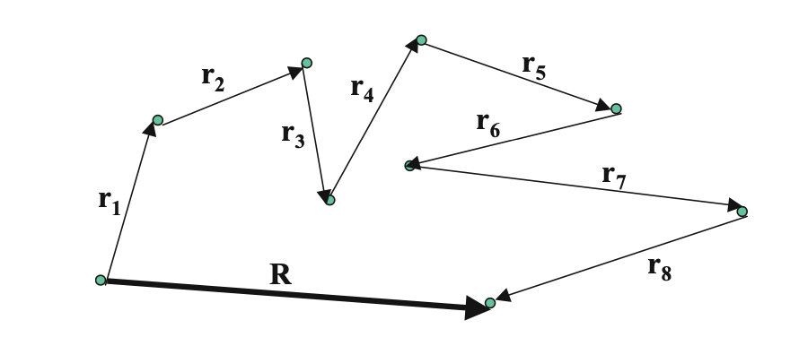Fig. 1. A random walk with 8 steps in 2-D.

As illustrated in Fig. 1, a random walk describes the process of taking a step of random size and direction from a specified point (origin), which is then repeated at the new arrival point for a specified number $n$ of steps. Each step is thus represented by a (in this case a 2-D) vector \(\vec{r}_i\) where the index \(i = 1,\dots,n\) labels the step number.

In this framework, a natural question to ask is

• “What is the direction and length of the displacement vector \(\vec{R}\) after the completion of a random walk consisting of $n$ steps?”

Since the total displacement vector is sum of random individual step vectors, the direction and length of \(\vec{R}\) is also random. Therefore, we can only make statistical statements about the properties of this vector, e.g by repeating a large number of random walks with the same number of steps. Only in this way, we can gain meaningful insights about the properties of \(\vec{R}\). The first fundamental observation we can make in this direction is the expectation value of the displacement vector: if we were to repeat many random walks, each of \(\vec{R}\) obtained from these experiments will point in any direction (in the 2-D Euclidean space) with equal likelihood, therefore on average they will “cancel” each other resulting with

\[\begin{equation}\label{edv} \mathbb{E}[\vec{R}] = 0. \end{equation}\]

Similarly, each step vector \(\vec{r}_i\) can also point in any direction with the same probability and therefore \(\mathbb{E}[\vec{r}_i] = 0\). The same conclusion can be reached from \eqref{edv} using the fact that each step is identical to each other:

\[\begin{equation}\label{eidv} \mathbb{E}[\vec{R}] = \mathbb{E}\left[\sum_{i = 1}^n \vec{r}_i\right] = n\, \mathbb{E}[\vec{r}_i] \implies \mathbb{E}[\vec{r}_i] = 0. \end{equation}\]

Besides being identical, the steps that constitute a random walk are independent of one another and therefore uncorrelated. In other words, we expect that on average the dot product of two different step vector to be vanishing:

\[\begin{equation}\label{indep} \mathbb{E}[\vec{r}_i \cdot \vec{r}_j] = 0, \quad\quad \forall\, i \neq j. \end{equation}\]

This makes intuitive sense by recalling that the dot product is a measure of the cosine angle, \(\cos\theta \in [-1,1]\) between two vectors and since after taking a step (of certain size), the next one can be in any direction (and size), on average we not expect to have a “bias” on their relative orientation. The independence of non-overlapping individual steps \eqref{indep} allow us to derive one of the most important statistical property of a random walk, namely the variance of the total displacement vector which is simply given by its norm squared

\[\begin{equation} \mathbb{V}[\vec{R}] \equiv \mathbb{E}\left[(\vec{R} - \mathbb{E}[\vec{R}])^2\right] = \mathbb{E}\left[\vec{R}\cdot \vec{R}\right]. \end{equation}\]

Noting \eqref{indep}, we then have

\(\begin{align} \nonumber \mathbb{V}[ \vec{R} ] &= \mathbb{E} \left[ \sum_{i = 1}^n \vec{r}_{i} \cdot \sum _{j = 1}^n \vec{r} _{j}\right] = \sum _{i,j = 1}^n \mathbb{E}[\vec{r} _{i} \cdot \vec{r} _{j} ], \\ \nonumber &= \sum _{i = 1}^n \mathbb{E}[\vec{r} _{i} \cdot \vec{r} _{i} ] + \sum _{i \neq j} \mathbb{E}[\vec{r} _{i} \cdot \vec{r} _{j} ], \\ \nonumber &= \sum _{i = 1}^n \mathbb{E}[\vec{r} _{i} \cdot \vec{r} _{i} ], \\ &= n\, b^2, \label{var} \end{align}\) where by definition $b$ denotes the mean norm of a single step:

\[\begin{equation}\label{bsq} b^2 \equiv \frac{1}{n} \sum _{i = 1}^n \mathbb{E}[\vec{r} _{i} \cdot \vec{r} _{i} ]. \end{equation}\]

As per \eqref{var}, the uncertaint (standard deviation) on the norm of the displacement vector increases proportional to square root of number of steps, \(\sqrt{n}\) that constitutes the random walk. As we will show later on, when a random walk process is used to model the price movements in the financial markets, the number of steps we considered so far corresponds to time. This is why the uncertainty in the future price movements increases proportional to the square root of time (a concept that is often referred to as “square root of time rule”). Notice that in deriving \eqref{var}, no information about the dimensionality of the ambient space (in which random walk takes place) is required. Therefore \eqref{var} holds in any dimension and is a fundamental property of random walks.

Another fundamental property of random walks that is worth mentioning is self-similarity: the statistical properties of random walk are always the same regardless of the degree of detail in which they are observed. In other words, a step in a random walk can be as well considered as the total displacement vector of a random walk with infinitesimal steps. Similarly, total displacement vector of a random walk can be itself considered as as a single step of a “larger” random walk process.

So far, we have derived first two moments (namely expectation value and the variance) of the probability distribution $p(\vec{R})$. In fact, utilizing the fundamental properties of a random walk we mentioned above, we can derive the probability distribution of the displacement vector $\vec{R}$ with the help of the central limit theorem (CLT) in the limit of $n \to \infty$. In particular, in a $d$ dimensional space, the probability distribution of the displacement vector can be shown to follow a normal distribution. Below, I will prove this for $d = 1$ (in this case $\vec{R}$ is actually a scalar I will denote by $R$) which is the case of interest in financial applications.

For this purpose, let’s assume that we start our random walk at the origin $R = 0$. The final displacement we have with respect to the origin after completing a random walk of $n$ step does depend on the number of steps $m$ we take to the right (or up) and to the left (down) which we can denote by $n-m$. Assuming we take a unit step with equal probability (as in a random walk) $p = 1/2$ in each direction, our final position after $n$ steps is thus $R = m - (n - m) = 2m - n$. To understand the probability distribution of the total displacement, we can think of each step as a Bernoulli (or binomial) trial with a Boolean outcome $\pm 1$ of probability $p = 1/2\,$ for $+1$ (up) and $q = 1 - p = 1/2\,$ for $-1$ (down). After taking $n$ steps (trails) the probability of taking $m$ steps to the right (or $n-m$ to the left) then is given by the binomial distribution:

\[\begin{equation}\label{bde} p(m,n) = \frac{n!}{m!\,(n-m)!} p^m q^{n-m} \end{equation}\]

with a mean and variance given by

\[\begin{equation}\label{bstat} \mathbb{E}[m] \equiv \bar{m} = n p, \quad\quad\quad \mathbb{V}[m] = n p q \end{equation}\]

so that $n, \mathbb{E}[m], \mathbb{V}[m] \sim \mathcal{O}(n) \gg 1$ in the large $n$ limit. As should be clear from \eqref{bstat}, we also typically expect $m, n-m \sim n/2$ and hence $\mathcal{O}(n) \gg 1$ as well. This should be intuitive because without a priori, we expect to make $m \sim n/2$ up steps when $n$ is large. In this limit, we can approximate the probability distribution utilizing Stirling’s formula/approximation as

\[\begin{equation}\label{bd} p(m,n) \simeq \left(\frac{n p}{m}\right)^m \left(\frac{n q}{n-m}\right)^{n-m} \sqrt{\frac{n}{2 \pi m(n-m)}}\left[1+\mathcal{O}\left(\frac{1}{n}\right)\right]. \end{equation}\]

To simplify this expression further, we define a small quantity $\epsilon = m - np \ll 1$ such that $ m = np + \epsilon$ and $n - m = n q - \epsilon$. We then utilize the Taylor expansion $\ln(1+y) = y - y^2 /2 + \mathcal{O}(y^3)$ to re-write the the logarithm of the first two terms in \eqref{bd} as

\(\begin{align} \nonumber \ln\left[\left(\frac{n p}{m}\right)^m \left(\frac{n q}{n-m}\right)^{n-m}\right] &= m \ln\left[\frac{np}{m}\right] + (n-m) \ln\left[\frac{n q}{n - m}\right],\\ \label{a1} &= -\frac{\epsilon^2}{2 n p q} + \mathcal{O}\left(\frac{\epsilon^3}{n^2}\right), \end{align}\) after a bit of algebra. Similarly, the third term in \eqref{bd} can be approximated as

\[\begin{equation}\label{a2} \sqrt{\frac{n}{2 \pi m(n-m)}} = \sqrt{\frac{1}{2 \pi n p q}}\left[1 + \mathcal{O}\left(\frac{\epsilon}{n}\right)\right]. \end{equation}\]

Notice that for the validity of the small $\epsilon$ expansions in \eqref{a1} and \eqref{a2}, we may expect $\epsilon$ to be at most $\mathcal{O}(\sqrt{n})$ so that corrections are negligible, $\propto \mathcal{O}(1/\sqrt{n})$, for large $n$. This implies that the formulas we provide here are valid for $m$ that is an order one factor of standard deviation $\sigma = \sqrt{npq}$ away from the mean $\mu = np$.

Finally, using exponentiation of \eqref{a1} and using it in \eqref{bd} together with \eqref{a2}, the large $n$ limit of \eqref{bde} read as

\[\begin{equation} p(m,n) \simeq \frac{1}{\sqrt{2 \pi n p q}}\mathrm{e}^{-(m-n p)^2 / 2 n p q} \end{equation}\]

which has the standard Gaussian form. To express the probability distribution in terms of the total displacement $R$, we recall $R = 2m - n$ and $p = q = 1/2$ for probabilities to get

\[\begin{equation}\label{pdR} p(R) \simeq \frac{2}{\sqrt{2\pi \mathbb{V}[R]}} \mathrm{e}^{-(R - \mathbb{E}[R])^2 / 2 \mathbb{V}[R]} . \end{equation}\]

Therefore, the total displacement $R$ from the origin has a normal distribution with mean $\mathbb{E}[R] = 0$ and variance $\mathbb{V}[R] = n$ as expected from a random walk process in $d = 1$ with a unit average step length $b^2 = 1$ as described by eq. \eqref{bsq}. The probability distribution in eq. \eqref{pdR} and its moments in eqs. \eqref{edv} and \eqref{var}, along with the self-similarity are the most fundamental properties of a random walk that clear the path for its application in finance.

Random walks for asset pricing

---

To finally develop an intuitive model of asset prices in the financial markets, we need to introduce the Markov property of a random processes which assumes that the future behavior of a stochastic process is only influenced by its current value, independent of the path taken to reach it. When we inject this property to financial risk factors such as stock prices, it follows that the subsequent values taken on by a given stock depend only on the current price and some external factors such as politics etc. but not on past prices.

To derive a model stock prices $P(t)$, we assume it is represented by a Markov process that consist of a random (stochastic) and deterministic component called the drift.

1. Modeling the stochastic component

We can adopt the $d = 1$ dimensional random walk process to model the random component as required to capture upward and downward changes in stock prices. Assuming that we observe the stock price changes at a fixed time intervals $\Delta t$ (minutely, hourly, daily and weekly etc.) over a time interval between today $t$ and at a future time $T$, the number of steps $n$ in the random walk describing the stock price movements is proportional to the entire time interval over which it takes place:

\[\begin{equation}\label{stime} T - t = n\, \Delta t . \end{equation}\]

Now, an important decision we need to make is about the real parameter/quantity that we choose to model by a random walk. As a first guess, let’s consider the market price of an asset. If the market price itself were a random walk then as a result of the self-similarity property, the price changes would also be random walks. To illustrate this, consider the price difference between $t = 0$ and a final time $t = n$:

\[\begin{equation}\label{Prd} P_n - P_0 = (P_1 - P_0) + (P_2 - P_1) + \dots + (P_n - P_{n-1}) \equiv \sum_{i = 1}^n \Delta P_i, \quad\quad \Delta P_i = P_i - P_{i-1}, \end{equation}\]

which certainly checks the first requirement that the “end-to-end” vector $P_n - P_0$ is the sum of small incremental price changes $\Delta P_i$. However, this would be problematic in terms of universally modelling different assets with eq. \eqref{Prd} as the price changes do not show such universality between for example an asset priced at 100 dollars and 1 dollar. To be able to model universally different assets, we may consider relative price changes:

\[\begin{equation}\label{Prr} \frac{P_n}{P_0} = \frac{P_1}{P_0} \frac{P_2}{P_1} \times \dots \frac{P_n}{P_{n-1}} \equiv \prod_{i=1}^{n} \frac{P_i}{P_{i-1}}, \end{equation}\]

which is clearly a product of relative price changes at each individual step. In this form, it is not a suitable candidate for a random walk as the total relative price movement is not a sum of the individual steps. The simplest way we can turn this expression to a sum is by taking the logarithm of both hand side,

\[\begin{equation}\label{lpr} \ln \left(\frac{P_n}{P_0}\right) = \sum_{i=1}^{n} \ln \left( \frac{P_i}{P_{i-1}} \right). \end{equation}\]

Eq. \eqref{lpr} finalizes the construction of the stochastic component by interpreting logarithm of the prices changes as random walk with iid random steps and the number of these steps being proportional to the duration of time during which the random walk takes place.

In analogy with the discussion we presented above, we then expect the total displacement $R = \ln [P(T)/P(t)]$ to be normally distributed with a vanishing expectation value and variance given by

\[\begin{equation}\label{lprd} \mathbb{E}\left[\ln \left(\frac{P(T)}{P(t)}\right)\right] = 0, \quad\quad \mathbb{V}\left[\ln \left(\frac{P(T)}{P(t)}\right)\right] = b^2 n \equiv \sigma^2 (T-t) \end{equation}\]

where we defined the volatility squared (using eq. \eqref{stime}) as

\[\begin{equation} \sigma^2 = \frac{b^2}{\Delta t} = \frac{1}{T-t}\mathbb{V}\left[\ln \left(\frac{P(T)}{P(t)}\right)\right]. \end{equation}\]

Eq. \eqref{lprd} expresses one of the fundamental points we advertised at the beginning of this post, namely the standard deviation of the logarithm of the price movements (or the square root of its variance) proportional to the square root of time!

Thanks to the self-similarity property of random walks, all infinitesimal changes in the logarithm of the price of an asset, over an infinitesimal time interval $\Delta t \to \mathrm{d} t$ is also normally distributed with a mean zero and variance given by:

\[\begin{equation}\label{vlprd} \mathbb{V}\bigg[\ln \left(\frac{P(t + \mathrm{d}t)}{P(t)}\right)\bigg] = \mathbb{V}\bigg[\ln \left(P(t + \mathrm{d}t)\right) - \ln \left(P(t)\right)\bigg] = \mathbb{V}\bigg[\mathrm{d}\ln(P(t))\bigg] = \sigma^2 \mathrm{d} t. \end{equation}\]

The stochastic differential process described by $\mathrm{d} \ln(P(t))$ is called a Wiener (or Brownian motion) process denoted by $W$. It is a process that changes randomly by a $\mathrm{d}W$ amount over a time interval $\sqrt{\mathrm{d}t}$. By definition, these changes are Gaussian distributed with a mean zero and variance proportional to the time, $\mathrm{d} t$ passed during the change. The shorthand notation for this statement is as follows:

\[\begin{equation}\label{W} \mathrm{d}\ln(P(t)) \sim \mathrm{d}W \sim X \sqrt{\mathrm{d}t},\quad\quad X \sim \mathcal{N}(0,1), \end{equation}\]

where $\mathcal{N}(a,b)$ notation denotes Gaussian (normal) distribution with mean $a$ and variance $b$ so that $\mathcal{N}(0,1)$ refers to standard normal distribution. On the other hand, the $\sim$ sign stand to indicate the way a quantity is distributed. In light of the definition in eqs. \eqref{W},\eqref{vlprd} and noting $\mathbb{E}\left[\mathrm{d}\ln(P(t))\right] = 0$, we can model the stochastic component for the infinitesimal changes in the log prices of an asset as

\[\begin{equation}\label{dlpr} \mathrm{d}\ln(P(t)) = \sigma\, \mathrm{d}W. \end{equation}\]

2. Modeling the drift term

Adding the classical component to the eq. \eqref{dlpr} is rather easy intuitively. If we want our one dimensional random walk process (of $R = \ln(P(T)/P(t))$) to parametrize the movements in the stock prices, we would expect it show a (positive) mean return in the long run such that the expected value of the total displacement $R$ is not equal to zero but rather grow with time. For infinitesimal movements in the logarithm of the asset prices, such a component can be introduced by adding a drift term in \eqref{dlpr} as

\[\begin{equation}\label{dlprf} \mathrm{d}\ln(P(t)) = \mu\, \mathrm{d} t + \sigma\, \mathrm{d}W, \end{equation}\]

where $\mu$ parametrize the rate of change in the log prices over an infinitesimal time interval $\mathrm{d} t$ in the absence of the random component $\mathrm{d} W \to 0$.

Notice that since we did not add any random component, the end to end displacement described by the $\ln(P(T)/P(t))$ still has normal distribution with variance given as in eq. \eqref{lprd} after the passage of time $T-t$. However, its expectation value (e.g its mean) is now given by

\[\begin{equation} \mathbb{E}\left[\ln\left(\frac{P(T)}{P(t)}\right)\right] = \mu \, (T-t). \end{equation}\]

The random walk we derived for the price movements can be generalized to include non-constant drift and volatility. For example using the relation \eqref{vlprd} for volatility and by absorbing its time dependence into its definition, we can generalize eq. \eqref{dlprf} with the help of eq. \eqref{W} as

\[\begin{equation}\label{gsp} \mathrm{d}\ln(P(t)) = \mu(P(t),t)\, \mathrm{d} t + X \sqrt{\mathbb{V}\left[\mathrm{d}\ln(P(t))\right]},\quad\quad X \sim \mathcal{N}(0,1). \end{equation}\]

This equation has the form of a stochastic diffusion process (also referred to as an Ito process) that sets the basis for more general random processes used to model market parameters:

\[\begin{equation}\label{gito} \mathrm{d} f(t) = a(f,t) \mathrm{d}t + b(f,t) \mathrm{d} W, \end{equation}\]

where $f$ is a random variable.

References

---

1. “Derivatives and Internal Models: Modern Risk Management”, Hans-Peter Deutsch and Mark W. Beinker .