Hedging and Global Minimum Variance Portfolio

In an earlier post, I have discussed the importance portfolio construction (by means of mean-variance optimization) with uncorrelated assets and its utility in mitigating potential investment losses. Here, I will briefly explore another useful practice in portfolio management: hedging, which can be considered a way of portfolio protection, often seen as important as portfolio appreciation.

What is Hedging?

The simplest way to understanding hedging is to think about it as a form of insurance but not in a literal sense. It is a strategy that can be considered to protect a portfolio against the negative financial consequences of an event that we might anticipate to occur. When carried properly, hedging does not reduce all the negative outcomes of the event, however it simply reduces the damage. It is a common practice utilized by portfolio managers and corporations to reduce their exposure to various financial risks.

At a high level, hedging against an investment risk refers to strategically using other financial instruments to offset the risk of any unexpected price movements in the former. In other words, investors hedge one investment by making a trade in another. Commonly this strategy is used among securities that have negative correlation, but the general idea can be implemented with positively correlated assets.

As an example, consider that we own shares of a stock A that is quite volatile. To protect ourselves from this downside risk, we can buy a derivative of the stock, such as a put (or sell) option which gives us the right to sell the stock in a specified time (or range) in the future. In this way we protect ourselves from large downside moves by paying a premium to purchase the option. In this example, we are reducing the risk for the purpose of reducing a potential loss and not for maximizing our profits. If the investment we are hedging against makes money, it means that we have also reduced our potential profits. However, if the investment loses its value, our hedge is successful in the sense that we have potentially reduced our losses.

To illustrate the idea mathematically, consider a portfolio of two assets. The expected portfolio return and variance is then given by

\[\begin{align} \nonumber \mathbb{E}[R_p] &\equiv \mu_p = \vec {w}^T \cdot \vec{\mu},\\ \label{var}\mathbb{V}[R_p] &\equiv \sigma_p^2 = \vec{w}^T \cdot ( {\bf \Sigma} \cdot \vec{w}), \end{align}\]

where $\vec{w} = [w_1, w_2]^T$ is weight vector, $\vec{\mu} = [\mu_1, \mu_2]^T$ is the vector representing the expected returns of each asset and the covariance matrix is given by

\[\begin{equation}\label{cov} {\bf \Sigma} = \begin{bmatrix} \sigma_1^2 & \,\rho\,\sigma_1 \sigma_2 \\ \,\rho\,\sigma_1 \sigma_2 & \sigma_2^2 \end{bmatrix} \end{equation}\]

with $\rho = \rho_{12} = \rho_{21}$ representing the (off diagonal) correlation between assets. Using \eqref{cov}, portfolio variance \eqref{var} for two assets can be explicitly written as

\[\begin{equation}\label{var2} \sigma_p^2 = w_1^2\, \sigma_1^2 + w_2^2\, \sigma_2^2 + 2 w_1 w_2\, \rho\, \sigma_1 \sigma_2 \end{equation}\]

Now consider the extreme case of perfect correlation $\rho = 1$. In this case, we can simply reduce the portfolio variance \eqref{var2} by taking an equal amount of short and long positions in the portfolio, $w_1 = -w_2$. This operation can be considered as example hedging the second asset against the first for the purpose of reducing the risk. Since we have equal amount of capital for long and short positions such a strategy is also referred as dollar-neutral strategy which is often adopted by hedge funds. For the example at hand, the portfolio variance reduces to

\[\begin{equation}\label{varr1} \sigma_p^2 = w_1^2 (\sigma_1 - \sigma_2)^2 = w_2^2 (\sigma_2 - \sigma_1)^2, \end{equation}\]

while our expected portfolio return is given by

\[\begin{equation}\label{mupr1} \mu_p = w_1 (\mu_1 - \mu_2). \end{equation}\]

Therefore, by taking an opposite position for two perfectly correlated assets, we can reduce the risk of the portfolio while potentially collecting a positive return (e.g for $\mu_1 > \mu_2 > 0$ with $\sigma_1 > \sigma_2$) that appears like a single net long position with a mean return $\propto (\mu_1 - \mu_2)$.

Now consider the opposite end of the “spectrum” corresponding to perfectly anti-correlated assets $\rho = -1$. In this case the portfolio variance is given by

\[\sigma_p^2 = (w_1 \sigma_1 - w_2 \sigma_2)^2\]

so the a smart choice to reduce variance is to take the same position $w_1 = w_2$ which is equivalent to \eqref{varr1}. In fact compared to the perfectly correlated example, we can situate ourselves in a better position in this case, as we can pump our expected returns further as compared to \eqref{mupr1}:

\[\mu_p \big|_{\rho = -1} = w_1 (\mu_1 + \mu_2),\]

for $\mu_1 > \mu_2 > 0$.

The examples I provided so far works as intended however notice that we have not enforced any constraints on the porfolio weights. In fact, the natural choice of constraint for the perfectly correlated example we discussed could be $w_1 + w_2 = 0$ whereas for the anti-correlated case we could have adopted $w_1 + w_2 = 1$ with $w_1 = w_2$ so that $w_1 = w_2 = 0.5$. On the other hand, these examples are toy examples that work on the extreme opposites of the correlation spectrum $\rho = [-1, 1]$ which is virtually non-existent in the real markets.

So the discussion we presented so far begs for a systematic approach that can guide us to better understand hedging strategy. For this purpose, we can take guidance from Markowitz’s portfolio theory. Recall that our main aim is risk reduction without referring to the mean returns of the portfolio. Therefore the simplest thing we can do is to seek for directions in the weight space that minimize the portfolio variance. Since the portfolio variance is a convex function of weights for $-1 < \rho < 1$, there should exist a weight combination that lands us to the global minimum. Such a point would appear as the global minimum variance portfolio in the risk-reward spectrum of the portfolio. I will illustrate this concept for a two asset porfolio with the constraint $w_1 + w_2 = 1$ for simplicity.

Global minimum variance portfolio vs Hedging

To detetmine the global minimum of \eqref{var2}, we first look at the critical points which can be easily obtained after a bit of algebra as:

\[\begin{equation}\label{cp} w_1^{*} = \frac{\sigma_2^2 - \rho \sigma_1 \sigma_2}{\sigma_1^2 + \sigma_2^2 - 2\rho \sigma_1 \sigma_2},\quad\quad w_2^{*} = \frac{\sigma_1^2 - \rho \sigma_1 \sigma_2}{\sigma_1^2 + \sigma_2^2 - 2\rho \sigma_1 \sigma_2}. \end{equation}\]

The points are guaranteed to be the minimum if the determinant of the Hessian matrix of the function \eqref{var2} is positive definite:

\[\begin{equation} H = \begin{bmatrix} \frac{\partial^2 \sigma_p^2}{\partial w_1^2} & \frac{\partial^2 \sigma_p^2}{\partial w_1 \partial w_2} \\ \frac{\partial^2 \sigma_p^2}{\partial w_2 \partial w_1} & \frac{\partial^2 \sigma_p^2}{\partial w_2^2} \end{bmatrix} \quad \Longrightarrow \quad \textrm{det}(H) = 4 \sigma_1^2 \sigma_2^2 (1 - \rho^2). \end{equation}\]

Notice that the determinant is positive as long as we are working with a realistic correlation range $-1 < \rho < 1$, between two assets.

To understand the relationship between hedging and the global minimum variance portfolio, let’s consider a risky asset with a monthly mean return $\mu_A = 3 \%$ with volatility $\sigma_A = 6\%$ and another less risky asset with $\mu_B = 1\%$ and $\sigma_B = 3\%$. Now consider a slightly more realistic scenarios of strong anti-correlation/correlation between these assets focusing on $\rho = [-0.8,0.8]$. We ask ourselves the quesiton: “How can we hedge the risk of holding only the asset A by considering a portfolio with the asset B?” For this purpose we can consider all the possible portfolio’s build up by these assets (focusing on $w_{A/B} \in [-0.5, 1.5]$) as shown in the risk-reward spectrum Figure 1.

---

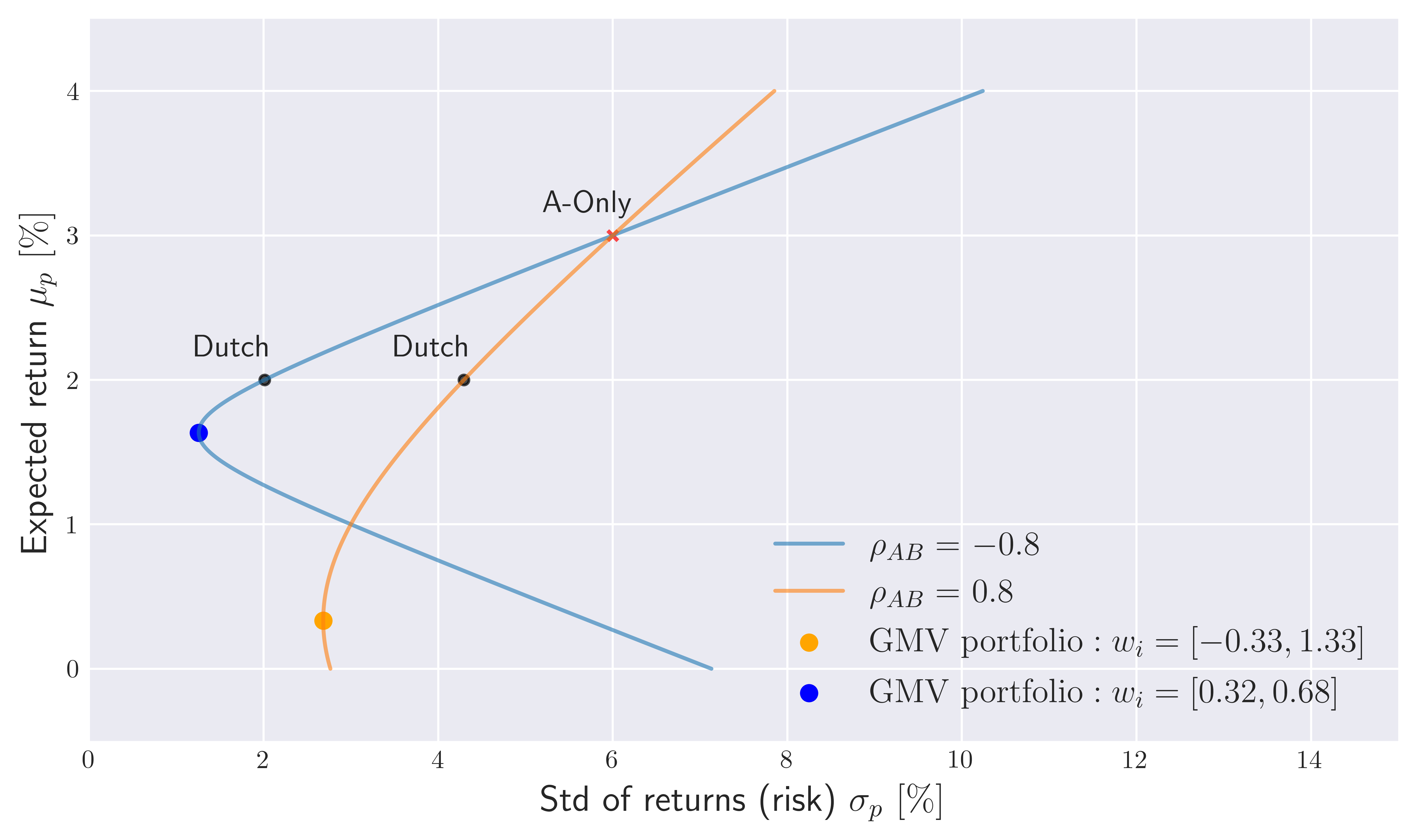Figure 1. Risk reward spectrum of two asset portfolio’s with $w_i \in [-0.5,1.5]$.

---

Notice that for both correlated and anti-correlated cases A-only portfolio’s with $w_i = [1,0]^T$ overlap on the risk-reward spectrum as in this case the correlation becomes simply irrelevant in the analysis. The diagram tells us that if we are simply interested in reducing the risk involved with A, we can adopt for example a fifthy-fifthy Dutch portfolio $w_i = [0.5,0.5]^T$ by holding equal amount of the assets. However, this choice would not be optimal as we we can further reduce the risk along the efficient frontier by reaching to the global minimum variance portfolio (GMVP) shown by colored points in Figure 1. Not surprisingly, there is no free lunch in the sense that these points also corresponds to lowest return rates within the efficient frontier. In fact, the global minimum variance portfolio can be considered as the onset of the efficient frontier which is generally defined by the top part of the Markowitz bullet.

In other words, by adopting the Dutch portfolio or the GMV portfolio, we can hedge our risk for our investment in the Asset A by investing some portion of our money to asset B. Which portfolio to pick depends on the investors preferences. Notice that for strongly negative correlated assets, if we are interested in minimizing our risk as much as possible, the wise choice would be going long for both assets by an almost thirty to seventy percent. This is consistent from our expectations for the toy examples we discussed in the beginning of this post. On the other hand, for strongly positive correlated assets, minimizing the risk requires to short sell the asset A by leveraging our position for the less risky asset B. As shown in Figure 1. this in turn does not provide us much reward however recall that our main aim here is to just reduce the risk of making an investment on only $A$. This result is also consistent with our earlier discussion: for positevely correlated assets, the optimal risk reduction can be achieved by taking opposite positions for the assets within the portfolio!

Python code that can be used to reproduce Figure 1. :

import numpy as np
import matplotlib as mpl

import matplotlib.pyplot as plt
from scipy.optimize import minimize

mpl.rcParams['text.usetex'] = True

#For inline plotting 
%matplotlib inline                 
%config InlineBackend.figure_format = 'svg'

plt.style.use("seaborn-v0_8-dark")


def get_pfolio_performance(mu,sigma,rho,w):
    
    '''Helper function to output expected return and std of a two asset
       portfolio given an array of expected individual asset returns (mu), 
       volatility (sigma), weights (w) and off-diagonal correlation (rho)
    '''
    
    mu_p = w.dot(mu)
    
    sigma_p = np.sqrt((w**2).dot(sigma**2) + 2 * w.prod() * sigma.prod() * rho)
    
    return mu_p, sigma_p

def global_min_var(s1,s2,corr):
    """Return two-asset portfolio weights for a given correlation and stds, 
       corresponding to the global minimum variance portfolio.
    """
    cov = np.array([[s1**2, s1*s2*corr],
                    [s1*s2*corr, s2**2]])
    res = minimize(
        fun=lambda x: (x.dot(cov)).dot(x),
        x0=[0.5,0.5], method = 'SLSQP', 
        constraints = {'type': 'eq', 'fun': lambda x: 1 - x.sum()},
        bounds = [(-0.5,1.5),(-0.5,1.5)]
        )
    
    return res.x

# array of asset returns and volatility
mu = np.array([3.,1.])
sigma = np.array([6.,3.])

# different correlation between assets
rho_vals = [-0.8,0.8]

# portfolio weights for global minimum variance portfolios 
wrho_p = global_min_var(6,3,rho_vals[1])
wrho_m = global_min_var(6,3,rho_vals[0])

# risk-reward valus for global minimum portfolios
gmvp_rhop_mu, gmvp_rhop_risk = get_pfolio_performance(mu,sigma, rho_vals[1], wrho_p)
gmvp_rhom_mu, gmvp_rhom_risk = get_pfolio_performance(mu,sigma, rho_vals[0], wrho_m)


####### Risk Reward spectrum for two asset portfolio #########

# Generate a grid of w_A values that we will iterate over
wa_min = -0.5
wa_max = 1.5
wa_space = np.linspace(wa_min, wa_max, 1000)

# empty array of risk-reward pairs
risk_vs_reward = np.full(shape = (1000,2), fill_value=0.)

# compute portfolio return and risk for each w_A and corresponding w_B
fig, axes = plt.subplots(figsize = (9,5))
for r_id, rho in enumerate(rho_vals):
    for idx, wa in enumerate(wa_space): 
    
        wb = 1 - wa 
    
        w = np.array([wa,wb])
    
        mu_p, sigma_p = get_pfolio_performance(mu,sigma,rho,w)
    
        risk_vs_reward[idx,0] = sigma_p
        risk_vs_reward[idx,1] = mu_p
    

    axes.plot(risk_vs_reward[:,0], risk_vs_reward[:,1], alpha =0.6,
              label = r'$\rho_{AB} =\,\, $'f"${rho_vals[r_id]}$")
    
############################################


# A-only portfolio for both correlation and Long-only Dutch
w_dict = {'A-Only': np.array([1,0]),'Long-Dutch': np.array([0.5,0.5])}
    
mu_ppm, sigma_ppm = get_pfolio_performance(mu,sigma,rho_vals[1],w_dict['A-Only'])

mu_pp, sigma_pp = get_pfolio_performance(mu,sigma,rho_vals[1],w_dict['Long-Dutch'])
mu_pm, sigma_pm = get_pfolio_performance(mu,sigma,rho_vals[0],w_dict['Long-Dutch'])

axes.scatter(sigma_ppm, mu_ppm, marker = 'x', s = 15, c = 'red', alpha = 0.7)

axes.scatter(sigma_pp, mu_pp, marker = 'o', s = 15, c = 'k', alpha = 0.7)
axes.scatter(sigma_pm, mu_pm, marker = 'o', s = 15, c = 'k', alpha = 0.7)

axes.annotate('A-Only', xy = (sigma_ppm-0.8,mu_ppm+0.16), size = 12)
axes.annotate('Dutch', xy = (sigma_pp-0.8,mu_pp+0.16), size = 12)
axes.annotate('Dutch', xy = (sigma_pm-0.8,mu_pm+0.16), size = 12)

#########################################

axes.scatter(gmvp_rhop_risk,gmvp_rhop_mu,
             c = 'orange', label = r'$\textrm{GMV portfolio}: w_i = [-0.33, 1.33]$')
axes.scatter(gmvp_rhom_risk,gmvp_rhom_mu,
             c = 'blue', label = r'$\textrm{GMV portfolio}: w_i = [0.32, 0.68]$')

axes.set_xlabel(r'Std of returns (risk) $\sigma_p\,\, [\%]$', fontsize = 14)
axes.set_ylabel(r'Expected return $\mu_p\,\, [\%]$', fontsize = 14)

axes.set_xlim(0,15)
axes.set_ylim(-0.5,4.5)

axes.grid()
axes.legend(loc = 4, fontsize = 13)