Binomial distribution

Binomial distribution

---

Binomial outcomes such as yes/no, spam/not spam, 0/1 lie at the heart of analytics since they play important roles on decision taking or other processes. A central concept in understanding Binomial distribution is a set of trials (a single of which is called a Bernoulli trial/experiment) each having boolean valued outcome with definite probabilities.

For example consider flipping a coin 10 times which is a Binomial experiment with 10 trials, each having two outcomes: heads or tails. Another example is asking 100 people if they watched the news in a not so special day. In this case the outcomes of either watched or not watched the news and since it is a regular day, one may assign equal probability $p = 0.5$ for the success (watched) and failure (not watched) $q = 1-p = 0.5$ of each trial (asking one person). However, having equal probability for the outcomes is not necessary as far as the probabilities of the outcomes sum up to one, $p+q = 1$. As an example in this direction, consider the following problem:

If the probability of a click (on web) converting to a sale is 0.02, what is the probability of observing 0 sales in 200 clicks?

Clearly, in this case the probability of outcomes are not equal: while a click to no sale has probability of $98\, \%$, the mutually exclusive event of a click producing a sale have small chance of only $2\,\%$. Despite this difference, the structure of this problem is the same as compared to the other examples we mentioned above and hence it can be considered within the framework of a Binomial experiment.

In general, a binomial experiment is an experiment that satisfies the following conditions:

1. A fixed number $n$ of trials.
2. Each trial is independent of others.
3. Each trial has only two outcomes.
4. The probability ($p$ and $q$) of each outcome (success/failure or 1/0 etc.) remains constant from trial to trial.

Binomial distribution help us to analyze the probability of the questions or problems that satisfy these conditions, similar to the examples I provided above.

Stated in a formal way, in statistics, binomial distribution with parameters $n$ and $p$ describes a discrete probability distribution of the number of successes in a sequence of $n$ independent Bernoulli trials, each asking yes/no questions with its own Boolean valued outcome of success with probability $p$ or failure with probability $q = 1 -p$.

Probability distribution function

Mathematically, if a random variable $X$ follows a Binomial distribution with parameters $n \in \mathbb{N}$ and $p \in [0,1]$, we write $X \sim B(n,p)$. The probability of obtaining $k$ successes (with the same rate of probability $p$) in a sequence of $n$ Bernoulli trials is given by the discrete probability distribution function $f$:

\[\begin{equation}\label{bpdf} \textrm{Prob}(X = k) \equiv f(k) = \frac{n!}{k!\,(n-k)!}\, p^k \, (1-p)^{n-k}, \end{equation}\]

for $k = 0,1,\dots,n$. The pre-factor that is given in terms of factorials is the binomial coefficient that gives the name to the distribution. In particular, we can understand this formula as follows. Consider a sequence of $n$ Bernoulli trials in which the first $k$ trials are “successes” and the remaining $n-k$ result in “failure”. The probability of obtaining this sequence is clearly $p^k\,q^{n-k} = p^k\, (1-p)^{n-k}$. However, does the order of obtaining “successes” and “failures” important? In fact, it does not. Since each trial is independent with the probability of outcomes remaining constant between them, any sequence of $n$ trials with $k$ “successes” and $n-k$ “failures” have the same probability above, irrespective of the relative positions of “successes” and “failures” in the sequence. The combinatorial pre-factor defined by

\[\begin{equation}\label{cnk} C(n,k) \equiv \binom{n}{k} = \binom{n}{n-k} = \frac{n!}{k!\,(n-k)!} \end{equation}\]

counts the number of different ways we can obtain $k$ “successes” (or equivalently $n-k$ “failures”) in a sequence of $n$ trials. The binomial distribution is concerned with the probability of obtaining any of these sequences and therefore the probability of obtaining one of them $p^k\, (1-p)^{n-k}$ must be weighted by a factor of $\binom{n}{k}$.

Statistical properties of Binomial distribution

Having the probability distribution at hand, we can derive moments (e.g mean and variance etc.) of the Binomial distribution. In particular the expectation value and variance of $k$ is given by:

\[\begin{align} \nonumber \mathbb{E}[k] &= \sum_{k = 0}^{n} k\, f(k),\\ \label{spk} \mathbb{V}[k] &= \mathbb{E}[k^2] - \mathbb{E}[k]^2 = \sum_{k = 0}^{n} k^2\, f(k) - \mathbb{E}[k]^2. \end{align}\]

To derive an expression for these quantities in terms of the parameters $n$ and $p$ of the Binomial distribution we are going to utilize a neat trick, (not so surprisingly) based on the Binomial expansion:

\[\begin{equation}\label{be} (p + q)^n = \sum_{k = 0}^{n} f(k) = \sum_{k = 0}^{n} C(n,k)\, p^k q^{n-k}. \end{equation}\]

Notice that in light of the Binomial distribution ($q = 1 - p$) this expression equals to unity, just implying the fact that the sum of the distribution function over all possible $k$ values must add up to 1. The trick I mentioned is all about bringing factors of $k$ on the right-hand side of the equation \eqref{be} by taking an appropriate number of derivates on both sides. For example consider the following

\[\begin{equation} p \frac{\mathrm{d}}{\mathrm{d}p} (p + q)^n = \sum_{k = 0}^{n} k\, C(n,k)\, p^k q^{n-k} = \sum_{k = 0}^{n} k f(k) \end{equation}\]

which is exactly the expectation value that we are looking for. Evaluating the derivative on the left-hand side we then send $q \to 1 - p$ to obtain the expectation value as

\[\begin{equation}\label{ek} n p = \sum_{k = 0}^{n} k f(k) = \mathbb{E}[k]. \end{equation}\]

Using essentially the same trick, we now look at expression

\[\begin{equation} p^2 \frac{\mathrm{d}^2}{\mathrm{d}p^2} (p + q)^n = \sum_{k = 0}^{n} k(k-1)\, C(n,k)\, p^k q^{n-k}. \end{equation}\]

Taking the derivatives on the left-hand side gives

\[\begin{equation} n(n-1)\,p^2\, (p+q)^{n-2} = \sum_{k = 0}^{n} k(k-1)\, C(n,k)\, p^k q^{n-k} \end{equation}\]

which is valid for any $p$ and $q$. Setting again $q = 1 - p$, we obtain

\[\begin{equation} n(n-1)\,p^2 = \sum_{k = 0}^{n} k(k-1)\, C(n,k)\, p^k (1-p)^{n-k} = \sum_{k = 0}^{n} k^2 f(k) - \mathbb{E}[k]. \end{equation}\]

Using eq. \eqref{ek}, this relation gives

\[\begin{equation} \sum_{k = 0}^{n} k^2 f(k) = n^2\,p^2 - n p^2 + np. \end{equation}\]

Then the variance defined in eq. \eqref{spk} (again using eq. \eqref{ek}) can be obtained as

\[\begin{equation} \mathbb{V}[k] = np\, (1 - p) = n p q. \end{equation}\]

Higher cumulants of the Binomial distribution can be obtained by applying higher derivatives (of $p$) on the expression \eqref{be} together with factor of appropriate powers of $p$.

The Gaussian approximation to Binomial distribution

Remarkably, in the limit of large number of trials, $n \gg 1$, the binomial distribution can be well approximated by a normal distribution. This result is a direct consequence of the Central Limit Theorem (CLT), which states that the sum of a large number of independent, identically distributed random variables (like the individual Bernoulli trials in a binomial distribution) will tend to follow a normal distribution. In an earlier post, I have shown a derivation of this correspondence by modelling 1-d random walk that exhibit a large number of steps as binomial distribution. I do not intend to repeat these mathematical details here. Instead, I would like to illustrate the approach of the Binomial distribution to a normal distribution with Python.

First, I would like to define a function for the Binomial probability distribution as a function of $n$ trials and $k$ successes with a given probability $p$. For this purpose, I find it useful to take a dynamic programming approach which is especially useful when the number of trials $n$ and the number of succeses $k$ are large because in this case, a brute force approach of defining the corresponding mathematical expression (e.g eqs. \eqref{bpdf} and \eqref{cnk}) would be computationally suboptimal.

To set the stage for dynamical programming logic, let’s re-write (using eq. \eqref{cnk}) the probability to obtain $k$ success (with a given probability $p$) in $n$ trials as given by the binomial distribution in eq. \eqref{bpdf}:

\[\begin{align} \nonumber \textrm{P}(n,k) &\equiv \binom{n}{k}\, p^k \, (1-p)^{n-k},\\ \label{bp}&= \left[\binom{n-1}{k-1} + \binom{n-1}{k}\right] p^k \, (1-p)^{n-k}, \end{align}\]

where in the second line we utilized the recurrence relation of binomial coefficients. Noting the original definition of the probability in the first line of eq. \eqref{bp}, we can then derive a recurrance relation for the probability to have $k$ success in $n$ trials as

\[\begin{align}\label{bpr} \textrm{P}(n,k) = \textrm{P}(n-1,k-1)\, p + \textrm{P}(n-1,k)\,(1-p). \end{align}\]

In other words, the probability of interest can be decomposed into sub-problems of

• The probability of having $k-1$ successes in the first $n-1$ trial and also succeeding on the $n$th trial (the first term).
• The probability of having $k$ success in the first $n-1$ trial and failing in the last trial (the second term).

Notice that in the special case of $k = 0$ (no success in $n$ trials), the recurrance relations simplifies since having a negative success is meaningless

\[\begin{align}\label{bprs} \textrm{P}(n,0) = \textrm{P}(n-1,0)\,(1-p). \end{align}\]

On the other hand, you might wonder the probability $\textrm{P}(0,0)$ as well which corresponds to obtaining 0 success in 0 trials. This event does happen with a unique certainty of doing nothing and therefore have a probability of one, $\textrm{P}(0,0) = 1$. This relation, along with the eq. \eqref{bprs}, is crucial for the dynamical programming logic as it allows the recursive relation to work properly, ensuring to build more complex cases using this simple base case. Building on these ideas, dynamic programming approach to the binomial probability distribution can be implemented in Python as:

import numpy as np
   
def binom_prob(n,k,p):

    # Validate inputs 
    assert isinstance(n, int) and n >= 0, "n must be a non-negative integer"
    assert isinstance(k, int) and k >= 0, "k must be a non-negative integer"
    assert isinstance(p, float) and 0.0 <= p <= 1.0, "p must be a float between 0 and 1"
    
    # Initialiaze a the probability table using numpy arrays
    p_table = np.zeros((n + 1, k + 1))

    # base case of n = 0, k = 0 with probability 1
    p_table[0][0] = 1.0

    #loop through n and k to fill the table 
    for i in range(1,n+1):
        
        p_table[i][0] = p_table[i-1][0] * (1-p) # cases with k = 0 for all n = 1,.. according to the recursion relation

        # loop through k = 1,... to update the probability table using the recursion relation
        for j in range(1, min(i,k) + 1)

            p_table[i][j] = p_table[i-1][k-1] * p + p_table[i-1][k] * (1-p)

    return p_table[n][k]

We can put the function to a simple test, considering the probability of getting two odd numbers when throwing a fair dice 3 times. In this case, there are 3 binomial experiments with the favorable outcome described by the following set: ${\textrm{OOE}, \textrm{OEO}, \textrm{EOO}}$ and the corresponding space of not favorable binomial experiments: ${\textrm{OOO}, \textrm{EEE}, \textrm{EEO}, \textrm{OEE}, \textrm{EOE}}$. Therefore, out of total of 8 binomial experiments, 3 ends up with two odd numbers giving us $P(3,2) = 3/8 = 0.375$. The same conclusion can be reached via the first line of eq. \eqref{bp}, noticing that probability of success, i.e getting an odd number each time you roll a die is $p = 1/2 = 0.5$.

prob = binom_prob(3,2,0.5)
print(f"The probability to obtain 2 odd numbers in a 3 successive roll of fair dice: {prob:.3f}")

Output:

The probability to obtain 2 odd numbers in a 3 successive roll of fair dice: 0.375

It seems like binomial distribution function we defined using dynamic programming method work as intended.

Now that we have the binomial probabilities for any $n$ and $k$, we can show the approach of the distribution to a normal one focusing on a large number of trials, e.g $n = 100$. The following Python snippet can be used to illustrate this

import matplotlib as mpl
import numpy as np
from scipy.stats import norm
import matplotlib.pyplot as plt

mpl.rcParams['text.usetex'] = True
plt.rcParams['xtick.labelsize'] = 13
plt.rcParams['ytick.labelsize'] = 13

#For inline plotting 
%matplotlib inline                 
%config InlineBackend.figure_format = 'svg'
plt.style.use("seaborn-v0_8-dark")

# Example parameters with large n
n = 100  # Number of trials
p = 0.5 # Probability of success on each trial

# generate a list of binomial probabilities for all possible k values for a given n, i.e for k = 0,1,... <= n
probs_klist = list()
for s in range(n+1):
    
    # append to the list calling binom_prob at each iteration
    probs_klist.append(binom_prob(n,s,p))


# Mean and standard deviation for the Gaussian distribution
mu = n * p
sigma = np.sqrt(n * p * (1 - p))

# Generate k values
k_values = np.arange(len(probs_klist))

# Calculate the Gaussian distribution 
gauss_probs = norm.pdf(k_values, mu, sigma)

# Plotting the binomial distribution
plt.figure(figsize=(10, 4))
plt.bar(k_values, probs_klist, width=0.3, color='blue', alpha=0.6, label='Binomial Distribution')

# Plotting the Gaussian distribution
plt.plot(k_values, gauss_probs, color='red', linewidth=2, label='Gaussian Distribution')

# Adding labels and title
plt.title(f'Normal distribution vs Binomial Distribution $(n={n}, p={p})$')
plt.xlabel(r'Number of Successes\,$(k)$', fontsize = 13)
plt.ylabel(r'$P(n,k)$', rotation = 0, fontsize = 13, labelpad = 30)
plt.legend()
plt.grid()

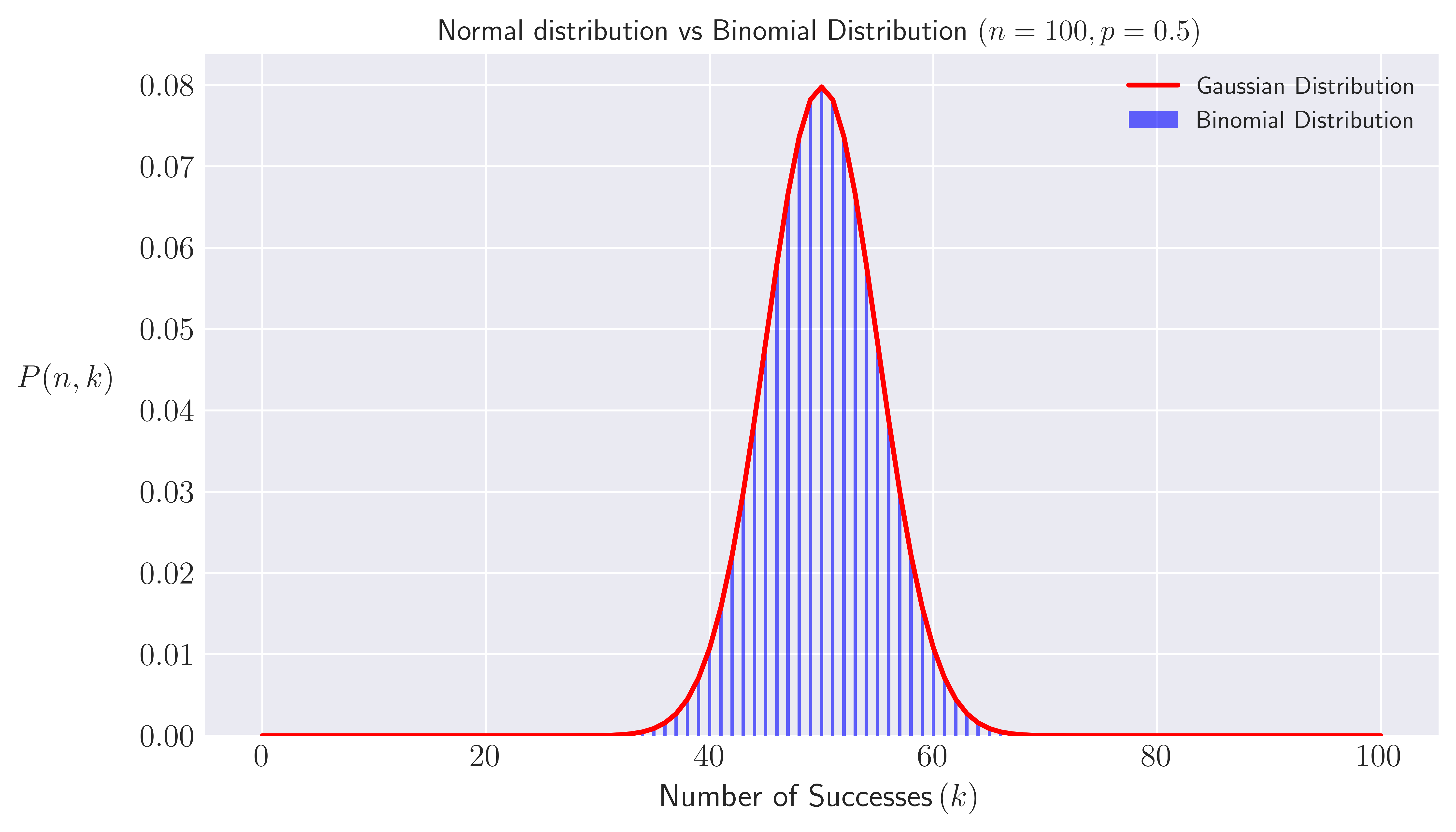Fig. 1. Bar plot of Binomial probability distribution for all $k \leq n$ for a large number $n = 100$ of Bernoulli trials vs normal distribution.

The figure above clearly shows that

\[\begin{equation} \textrm{P}(n,k) \sim \mathcal{N}(np, n p (1-p)). \end{equation}\]

Conclusions

---

The Binomial distribution help us gain insight on the statistical properties of successive events that exhibit boolean or binary outcomes. It forms the basis of many statistical inference methods used in Physics, Biology, Machine Learning and finance. In a seperate post, I will cover/introduce its use for options pricing in the finacial markets.