VaR and CVaR through Monte Carlo simulations
I discuss a commonly used VaR estimation method that utilizes Monte Carlo simulations.
In a series of earlier posts, I have introduced the concept of Value at Risk and it’s computation for a portfolio consist of a number of shares of a single asset assuming the latter follows a geometric brownian motion. This lead us to analytical formulate VaR of an investment in terms of the quantile of the log-return distribution of the asset, along with its drift and volatility. Focusing on real world stocks, I have then put these analytical formulas into a test for short term investments by comparing them with the historical method of VaR computation which does not rely on any assumption about asset’s (log) return distribution. I would like to start this post by mentioning the other practical methods of Value at Risk computation focusing on the Monte Carlo simulation method.
We start by reviewing the main idea behind each method assuming that each method is applied to portfolio consist of some number of assets. In general there are three main methods for VaR calculation for this purpose
- Delta-Normal (or Variance-covariance) method
- Historical method
- Monte Carlo method
Delta-Normal method: As its name may suggest, this method relies on some technical assumptions on the dependence on portfolio’s value with respect to the underlying assets in it. We will not get into the details here about the meaning of Delta in this context, but normal approximation should be intuitively clear. In this method, the main assumption is the normality of assets returns which implies that the portfolio returns (that is linear weighted combination of asset returns) are also normally distributed. Under this assumption, VaR (and CVAR) can be simply computed from the forecasts of portfolio returns and covariance matrix of returns. This method is sometimes also referred as variance-covariance method and also parametric method due its assumption on the distribution of portfolio returns. As this point, we note that one can also implement it using a more realistic distribution such as a t-distribution to take into account the observed fat tails of the asset/portfolio returns.
Historical method: This method applies current/desired positions to the past time-series data of assets in order to reconstruct the history of a hypothetical portfolio. Using the performence of this hypothetical portfolio, then the VaR and CVaR is obtained. In this sense, this method assumes the past portfolio performence will be indicative for the future. It has a powerful feature as compared to the parametric method, as no assumption is made about the distribution of portfolio returns. For a simple implementation of this method see my previous post.
Monte Carlo method: In the Monte Carlo method, one first decide on the stocastic process and its parameters that will be used to simulate the portfolio performance over a specified time horizon. At this step, the parameters (such as volatility, correlation and mean returns of assets) and their distributions can be derived from the historical data. Given the positions of each asset in the portfolio, we can then simulate many fictitious paths for the portfolio value to determine the VaR (and CVaR) at the boundary of the time horizon of interest. One may argue that Monte Carlo approach has the advantage of potentially capturing possible future movements in the portfolio value which could in principle work for any distribution that does not simply rely on normality assumption. The method, unfortunately, can be computationally heavy depending on the asset universe and the time horizon under consideration. This approach will be the focus for the rest of this post.
Monte Carlo Method for VaR and CVaR
To illustrate the Monte Carlo method at work for VaR and CVaR estimates, I will focus on a portfolio composed of three assets BP, NVDA and SBUX. In particular, I will focus on past two trading years of data between 2021-02-09 and 2023-02-09 to construct a maximum sharpe ratio portfolio within the Markowitz’s portfolio theory framework. For this purpose, I will utilize publicly available PyPortfolioOpt library within the asset class (see Appendix A) that I started developing in an earlier post. PyPortfolioOpt has many useful built-in methods that allows for portfolio optimization based on a variety of risk preferrences, for more details see the documentation. The following code snippet gives the returns and log-returns for the time frame we are interested in and the corresponding max sharpe ratio portfolio obtained via mean-variance analysis:
1
2
3
4
5
6
7
8
9
10
11
12
13
14
15
16
17
18
19
20
# we sort tickers in alphabetic order
# because the downloaded data will appear in that order
# this is important when we interpret weight allocations
tickers = sorted(['NVDA', 'SBUX', 'BP']) # stocks
end_date = pd.to_datetime('2023-02-10') # start and end date
start_date = end_date - dt.timedelta(days = 732)

# initialize the class and download price data
price_data = asset(tickers, start_date, end_date)
price_data.download()

# returns and log-returns
return_df, log_return_df = price_data.to_returns()

# get allocation weights for max sharpe ratio portfolio
weights = price_data.get_allocations()

for idx, ticker in enumerate(tickers):

    print(f"Allocation for {ticker}: w = {weights[idx]}")
Output:
[*********************100%%**********************]  3 of 3 completed
Price data downloaded for ['BP', 'NVDA', 'SBUX'] from 2021-02-08 00:00:00 to 2023-02-10 00:00:00
Allocation for BP: w = 0.5
Allocation for NVDA: w = 0.4333
Allocation for SBUX: w = 0.0667
The allocation weights obtained tells us that looking at the last two years of data, we should invest half of our money to BP and roughly $43 \%$ to NVDA and $7 \%$ to SBUX if we want to maximize sharpe ratio based on this historical data. Having obtained portfolio weights, we can keep track of the time evolution of the portfolio value for an initial investment of 1000 dollars (e.g 500 USD for BP, 430 USD for NVDA and 70 USD for SBUX) over a specified time horizon using Monte Carlo Simulation techniques. For this purpose, I have implemented a mc_sim() method that takes in the number of desired simulaton paths mc_sims, current portfolio value current_pval (e.g 1000 USD) to return portfolio value at the terminal time for all the paths. The method has an optional plot argument that is set to True by default to plot the resulting portfolio value paths. It relies heavily on the Cholesky decomposition/factorization of the historical covariance matrix. In simple terms, Cholesky decomposition allow us to determine the “square root” of the covariance matrix of asset returns which we can utilize to generate correlated asset returns from independent ones sampled say from the Gaussian distribution. The resulting asset returns then can be weighted by the allocations we derived and aggregated appropriately to determine the portfolio value over the time horizon of interest. This is the essential utility of mc_sim() under the hood:
1
port_val_sims = price_data.mc_sim(1000, current_pval=1000, plot = True)
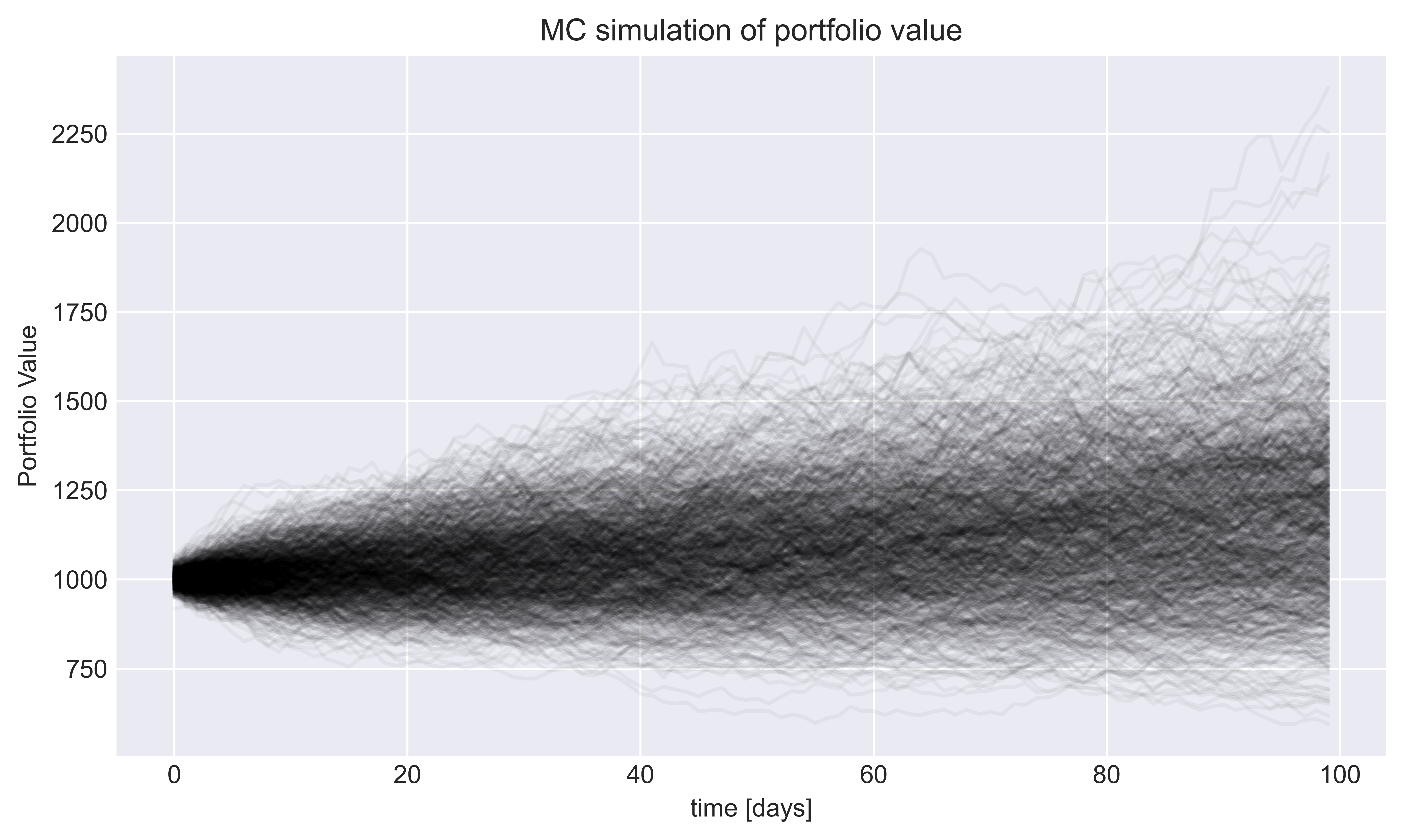 Figure 4. Monte Carlo simulations of max sharpe ratio (long-only) portfolio containing
 'BP', 'NVDA', 'SBUX' over 100 days. We constrained the weights on $w_i \in [0.01,0.5]$ for diversification. For this plot we ran 1000 simulations.
The different paths the portfolio value can take over a 100 day time horizon is shown in Fig 4. Once we have the distribution of the final portfolio values in the last time step corresponding to the right-most hand side of this plot. In particular, we can compute $1-c$ quantile $Q_{1-c}$ of this end point distribution which will inform us about a potential bad scenario at this confidence level (e.g $100 c\, \% = 95\, \% $) where our portfolio value declines. Then the value at risk can be determined by substracting this value from the initial investment (or portfolio value) which we assumed to be 1000 USD. On the other hand, expected shortfall of the portfolio value can be obtained by averaging over portfolio values that satisfy $PV < Q_{1-c}$. To implement the VaR and CVaR estimates within this Monte Carlo framework, I have extended and updated the risk class I introduced in a former post which can be found in Appendix B. VaR and CVaR estimates obtained in this way are shown in the code snipped below:
1
2
3
4
5
6
7
in_pval = 1000 # initial investment
dt = 100 # time horizon, actually necessary for historical method
fin_pvals = port_val_sims # portfolio values at last time slice
port_ret = price_data.get_portfolio_returns() # portfolio returns using get_portfolio_returns() method of `asset` class
risk_mc = risk(np.log(1+port_ret), dt, in_pval, fin_pvals)

print(f"Max sharpe ratio portfolio {tickers}, VaR = {risk_mc.mc_var():.3f} and CVaR = {risk_mc.mc_cvar():3f}")
Output:
Max sharpe ratio portfolio ['BP', 'NVDA', 'SBUX'], VaR = 175.344 and CVaR = 243.869These results tell us that with $95 \%$ confidence, our portfolio won’t lose more than 175 USD in value on a 1000 initial capital over 100 days. If it loses its value, the worst case scenario corresponds to a loss of 244 US in value within the same time horizon.
References
1. “Derivatives and Internal Models: Modern Risk Management”, Hans-Peter Deutsch and Mark W. Beinker .
Appendix A: asset class
1
2
3
4
5
6
7
8
9
10
11
12
13
14
15
16
17
18
19
20
21
22
23
24
25
26
27
28
29
30
31
32
33
34
35
36
37
38
39
40
41
42
43
44
45
46
47
48
49
50
51
52
53
54
55
56
57
58
59
60
61
62
63
64
65
66
67
68
69
70
71
72
73
74
75
76
77
78
79
80
81
82
83
84
85
86
87
88
89
90
91
92
93
94
95
96
97
98
99
100
101
102
103
104
105
106
107
108
109
110
111
112
113
114
115
116
117
118
119
120
121
122
123
124
125
126
127
128
129
130
131
132
133
134
135
136
137
138
139
140
141
142
143
144
145
146
147
148
149
import yfinance as yf
import numpy as np
import pandas as pd
from scipy.stats import skew, kurtosis
from pypfopt.efficient_frontier import EfficientFrontier

class asset:

    '''Class to download and process asset price data
       TO DO: More methods for preprocessing, statistics, plotting and mean-variance optimization etc.. '''
    def __init__(self,stocks,start,end):

        self.stocks = stocks
        self.start = start
        self.end = end

        self.price_data = None
        self.return_df = None
        self.log_return_df = None
        self.weigths = None

    def download(self):

        self.price_data = yf.download(self.stocks, self.start, self.end)

        if 'Close' not in self.price_data.columns:

            raise ValueError('Price data download failed or the ticker does not have close price data for the specified dates')

        else:

            print(f'Price data downloaded for {self.stocks} from {self.start} to {self.end}')

    def to_returns(self):

        '''Method to compute simple and log returns'''

        if self.price_data is None:

            raise ValueError('"Price data not downloaded. First download price data using .download() method')


        self.log_return_df =  np.log(1 + self.price_data['Close'].pct_change()).dropna()
        self.return_df = self.price_data['Close'].pct_change().dropna()

        return self.return_df, self.log_return_df

    def summary_stats(self):

        '''Get descriptive statistics of returns, adding skewness and kurtosis to the list'''

        if self.return_df is None:

            raise ValueError('Returns are not calculated, first run .to_returns()')

        # calculate stats on log returns
        stats_df = self.log_return_df.describe()

        stats_df.columns = self.log_return_df.columns + '_r'

        stats_df.loc['skew'] = skew(self.log_return_df)
        # fisher flag false --> # kurtosis is not w.r.t normal dist. where kurtosis = 3.
        stats_df.loc['kurtosis'] = kurtosis(self.log_return_df, fisher = False)

        return stats_df

    def get_allocations(self, type = 'max_SR'):

        '''Get the asset allocations for a given return dataframe and a specified risk/reward preference'''

        # historical mean returns and covariance for the specified time frame
        mean_returns = self.return_df.mean()
        covariance = self.return_df.cov()

        # Initialize the efficient frontier class from PyPortfolioOpt
        ef = EfficientFrontier(mean_returns, covariance, weight_bounds=(0.01,0.5))

        if type == "max_SR":

            # get max sharpe ratio allocation weights: a dictionary with ticker names as keys
            ef.max_sharpe(risk_free_rate=0.)
            max_sr_weights = ef.clean_weights()

            # Render the allocations as an array
            self.weights = np.array([val for key, val in max_sr_weights.items()])

            return self.weights

    def get_portfolio_returns(self):

        ''' Output portfolio returns using the simple return dataframe'''
        if self.weights is None:
            raise TypeError('Calculate allocations for the assets first, using .get_allocations()')

        return (self.return_df * self.weights).sum(axis = 1)


    def mc_sim(self, mc_sims, current_pval = 1., plot = True):

        if self.weights is None:

            raise ValueError('Compute the allocations first using get_allocations()')

        self.mc_sims = mc_sims # number of simulations
        T = 100 # time horizon in days

        mean_returns = self.return_df.mean()
        covariance = self.return_df.cov()

        #Cholesky decomposition of covariance matrix
        L = np.linalg.cholesky(covariance)

        # mean returns of assets, T x D, D = number of assets
        mean_Mat = np.full(shape = (T,len(self.weights)), fill_value=mean_returns)

        # variable to store portfolio simulations, T x number of simulations
        portfolio_sims = np.full(shape = (T,self.mc_sims), fill_value=0.0)

        # current portfolio value, default is set to 1.
        initial_portfolio_val = current_pval

        for sim_id in range(self.mc_sims):

            #sample random (uncorrelated) variables
            Z = np.random.normal(size = (T, len(self.weights)))

            # generate correlated log returns of assets
            daily_log_ret = mean_Mat + np.inner(Z,L) # L.Z is T x D

            # returns
            daily_ret = np.exp(daily_log_ret) - 1

            # for each simulation compute the price evolution for each T
            portfolio_sims[:,sim_id] = np.cumprod(1 + np.inner(daily_ret,self.weights)) * initial_portfolio_val

        if plot == True:

            fig, axes = plt.subplots(figsize = (12,5))

            axes.plot(portfolio_sims, alpha = 0.04, c = 'black')

            axes.set_ylabel('Portfolio Value')
            axes.set_xlabel('time [days]')

            axes.set_title('MC simulation of portfolio value')
            axes.grid()

        # return only the price distribution at the final time
        return portfolio_sims[-1,:]
Appendix B: risk class
1
2
3
4
5
6
7
8
9
10
11
12
13
14
15
16
17
18
19
20
21
22
23
24
25
26
27
28
29
30
31
32
33
34
35
36
37
38
39
40
41
42
43
44
45
46
47
48
49
50
51
52
53
54
55
56
57
58
59
60
61
62
63
64
65
66
67
68
69
70
71
72
73
74
75
76
77
78
79
80
81
class risk:

    ''' Class to implement VaR and CVaR computation'''

    def __init__(self, returns, dt, in_portfolio_val, fin_portfolio_val):

        ''' dt: time horizon for historical var/cvar method'''
        # initialize with a return series or dataframe
        if not isinstance(returns, (pd.Series, pd.DataFrame)):

            raise TypeError('Input returns must be pd.Series or pd.DataFrame object')

        self.dt = dt
        # Use log-returns as input for portfolio or assets
        self.returns = returns
        # initial investment / portfolio value
        self.in_portfolio_val = in_portfolio_val
        # portfolio value at the final time slice of various simulations
        self.portfolio_val = fin_portfolio_val

    def historical_var(self, alpha = 5):

        if isinstance(self.returns, pd.Series):

            var_lr = -np.percentile(self.returns, alpha)

            return self.in_portfolio_val * var_lr * np.sqrt(self.dt)

        elif isinstance(self.returns, pd.DataFrame):

            var_lr = -self.returns.aggregate(lambda x: np.percentile(x, alpha))

            return self.in_portfolio_val * var_lr * np.sqrt(self.dt)

    def historical_cvar(self, alpha = 5):

        neg_var = - self.historical_var(alpha)/(np.sqrt(self.dt) * self.in_portfolio_val)

        if isinstance(self.returns, pd.Series):

            below_var_returns = - self.returns[self.returns <= neg_var]

            return below_var_returns.mean() * np.sqrt(self.dt) * self.in_portfolio_val

        elif isinstance(self.returns, pd.DataFrame):

            var = -self.returns.apply(lambda x: x[x <= neg_var[x.name]].mean())

            return var * np.sqrt(self.dt) * self.in_portfolio_val

    def mc_var(self, alpha = 5):

        ''' Read portfolio value at the final time of the simulations
            to return its percentile at a given confidence level alpha'''

        # validate the input
        if isinstance(self.portfolio_val, np.ndarray):

            # maximum loss at 1-alpha CL: initial_investment - worst_final_portfolio_value @ 1-alpha CL
            return - np.percentile(self.portfolio_val, alpha) + self.in_portfolio_val

        else:

            raise TypeError('Input must be a np.array')


    def mc_cvar(self, alpha = 5):

        ''' Read portfolio value to output the expected shortfall (CVaR) for a given confidence level alpha '''
        var_pval_fin = -(self.mc_var(alpha)-self.in_portfolio_val)

        # validate the input
        if isinstance(self.portfolio_val, np.ndarray):

            below_var_bool = self.portfolio_val <= var_pval_fin

            return -self.portfolio_val[below_var_bool].mean() + self.in_portfolio_val

        else:

            raise TypeError('Input must be a np.array')