Value at Risk (VaR) and Conditional Value at Risk (CVaR)

In finance, the term risk generally refers to the potential financial losses may incur by a future event. Since the future is uncertain, risk is naturally related with the likelihood that an uncertain future event actually happens. Besides the probability of this event, the magnitude of the damage done is another important measure (the magnitude) of risk, in case the future event becomes real. For the purpose of controlling or minimizing the financial losses, the risk management departments of financial institutions therefore play an important role.

There are various types of risks depending on the nature of business/trades. Banks for example takes over risks in the form of market risk and credit risk.

Market (price) risk is stems from the uncertainty of the future development of market risk factors such as prices of shares, bonds or commodities, but also other parameters with a direct impact on the fair value of financial products, like FX or interest rates, inflation, volatilities or correlations between other market risk factors. In a portfolio for example, the risk could be the rise or fall of a certain share price. From this perspective, risk always depend on the particular position we take within a portfolio of assets. With this logic, it is not correct to characterize risk with the possibility of market risk factor fluctuations or the volatility of these factors as is done commonly.

On the other hand, credit risk describes the potential loss caused by the failure to pay or bankruptcy of a trading partner (counterparty risk) or issuer of securities (issuer credit risk) which are commonly summarized as credit risk or default risk. Besides market risk and credit risk there are other risk classes such as liquidity risk, operational risk, or legal risk that I will not dwelve into here.

In this post, I will refer to risk considering the present value of a portfolio as a reference. This portfolio could be consisted of securities (such as shares, bonds), derivatives and alike so that the risk associated with it can be mitigated by changing the positions (e.g. by hedging) of the risk factors that constitutes the portfolio.

The key figures to quantify the risk associated with a portfolio are Value at Risk (VaR) and Conditional Value at Risk (CVaR) (also referred to as expected shortfall) that are closely related to the statistical notions such as percentile and confidence level of a random variable with a specified probability distribution.

Confidence and Percentile vs Risk

---

Confidence Interval: A confidence interval of a random (stochastic) variable $X$ with a probability density function $p(X)$ can be described as the subset of the variable’s range that can be obtained with a specified probability $c$ that is referred to as confidence or level of confidence. A level $95\%$ confidence with $c = 0.95$ for example tells us that the probability that the value of the random variable lies inside the confidence interval is $95\%$ which automatically implies only $5 \%$ of the values the random variable takes lies outside this confidence interval. Considering that we are interested in the values of a random variable around a mean value $\mu$, the lower and upper bounds of a symmetric confidence interval can be defined as the values $a$ and $-a$ that satisfy the following condition:

\[c := P(\mu-a \leq x \leq \mu+a) = \int_{\mu-a}^{\mu+a} p(x)\,\mathrm{d}x .\]

Notice that by definition, the quantity $c$ above gives the cumulative probability $P$ that the value of the random variable $X$ lies within the range $x \in [\mu-a,\mu+a]$. We could as well be interested in the probability that the value of $X$ do not fall under a certain value. For this case, we consider a one-sided confidence interval and define the boundary $a$ as the value that satisfies

\[c := P(x > a) = 1 - P(x \leq a) = 1 - \int_{-\infty}^{a} p(x)\,\mathrm{d}x.\]

Percentile/Quantile: Given the definition of a confidence interval, it is easy to understand quantile/percentile of the distribution of the random variable $X$. The percentile can be defined as the boundary value $Q_c$ such that the value of the random variable is less than $Q_c$ with a level $c$ of confidence level:

\[P(x \leq Q_c) = \int_{-\infty}^{Q_c} p(x)\,\mathrm{d}x = c.\]

To explicitly obtain the percentile, we invert the cumulative probability function:

\[\int_{-\infty}^{Q_c} p(x)\,\mathrm{d}x = P(Q_c) - P(-\infty) = P(Q_c) = c, \quad\quad \Longrightarrow \quad\quad Q_c = P^{-1}(c)\]

For the example we discussed earlier, the boundary $a$ thus precisely corresponds to the $(1-c)$ percentile:

\[P(x\leq a) = 1 - c \quad\quad \Longrightarrow \quad\quad a \equiv Q_{1-c} = P^{-1}(1-c).\]

Using these definitions of confidence level, confidence interval and percentile we can define value at risk of a financial instrument or a portfolio with value $V$ at a given confidence level $c$.

Value at Risk (VaR): First and foremost, since the value of a portfolio is a function of the risk factors that are stochastic (random) in nature, so does the value of the portfolio itself. Note however that as a risk measure we are interested in the downside movements of a portfolio’s value (which is also stochastic). More precisely, value at Risk (VaR) in this case can be defined as the upper bound in the decline $\delta V$ of the portfolio’s value within a time interval of $\delta t$ that will not be exceeded with a confidence level $c$. In other words, we can implicitly define VaR using the cumulatif probability that the value of $\delta V$ will lie above $\delta V > -\textrm{VaR}$ with confidence $c$:

\[c := P(\delta V > - \textrm{VaR}(c)) \quad\quad \Longrightarrow \quad\quad c:= 1 - P(\delta V \leq - \textrm{VaR}(c)) = 1 - \int_{-\infty}^{-\textrm{VaR}(c)} p_{\delta V}(x)\, \mathrm{d}x,\]

where $p_{\delta V}(x)$ is the probability distribution function of $\delta V$. Value at Risk is then defined as the $1-c$ percentile of the distribution of $\delta V$:

\[\begin{align} P(\delta V \leq - \textrm{VaR}(c)) = 1 - c \quad \Longrightarrow \quad -\textrm{VaR}(c) = P^{-1}(1-c) = Q_{1-c}. \end{align}\]

So far, we discussed the VaR using the probability distribution of the change in the portfolio’s value $\delta V$. However, these changes are induced by the changes in the underlying risk factors. On the other hand, in practice we often first model stochastic processes and distributions of risk factors that make up the portfolio to infer the distribution and the stochastic process behind $\delta V$. Therefore, we might be interested to discuss VaR in terms of the risk factors (assets) that constitutes the portfolio.

Using the probability distribution of the risk factor instead of the probability distribution of the portfolio for the determination of the value at risk is only possible when $V$ is a monotonous function of the risk factor process $S$. If, for example, $V$ is a monotonously increasing function of $S$, we have

\[V(S) \leq V(a) \Leftrightarrow S \leq a\]

such that $V$ lies below the confidence interval bound for the portfolio if and only if $S$ lies below the confidence interval bound for the risk factor. The VaR of the portfolio is then the difference between the portfolio’s current value and the value of the portfolio when the risk factor lies at the lower bound $a$ of the confidence interval: $\textrm{VaR}(c) = V(S) - V(S = a)$. Similarly, when the portfolio’s value is monotonously decreasing function of the risk factor: $V(S) \leq V(\tilde{a}) \Leftrightarrow S \geq \tilde{a}$ and the portfolio VaR is the difference between the current value of the portfolio and the portfolio’s value when the upper boundary $\tilde{a}$ of the confidence interval of the risk factor is attained: $\textrm{VaR}(c) = V(S) - V(S = \tilde{a})$.

To summarize, if V is a monotonous function of the risk factor, the value at risk of the portfolio is

\[\begin{equation} \textrm{VaR}_V(c) = V(S) - \min\left[V(S = a), V(S = \tilde{a})\right] \end{equation}\]

Therefore, the one-sided confidence interval for the risk factor which is bounded from above determines the VaR for portfolios whose value declines with increasing underlying prices. Analogously, the one-sided confidence interval with a lower bound determines the value at risk for those instruments (or portfolios) whose prices rise with the rising price of the underlying. The values of many instruments like bonds, futures, and most options are monotonous functions of their risk factors. Portfolios which are not monotonous functions of their underlyings must be either stripped into their component elements which are monotonous functions of their underlyings or the distribution of V itself and its confidence interval must be determined directly. The confidence intervals of the risk factors are no longer of assistance in this case.

In addition to VaR there are other concepts used in the financial markets to quantify risk. Two risk measures mainly used in the asset management industry are conditional value at risk (CVaR or expected shortfall) and shortfall probability.

CVaR: VaR only tell us about the boundary (limit) of our losses at a certain confidence level but does not refer to more extreme losses beyond that confidence level. The conditional VaR precisely fill this gap by quantifying our expected losses beyond this confidence level. In other words, it is a conditional expectation value of our losses $\delta V$ given that $\delta V < - \textrm{VaR}(c)$:

\[\begin{equation} \textrm{CVaR} = \mathbb{E}[\delta V | \delta V < - \textrm{VaR}(c)] = - \int_{-\infty}^{- \textrm{VaR}(c)} x\, p_{\delta V}(x)\, \mathrm{d}x. \end{equation}\]

On the other hand, the shortfall probability gives us the probability that the change in portfolio value $\delta V$ is below a pre-specified amount. In a way, this is complementary to the Value at Risk: for VaR we are given the probability and calculate the loss, which will not be exceeded with this given probability; for shortfall probability we are given the loss and calculate the probability for this (or a larger) loss to occur. In other words, the shortfall probability belonging to a given loss equal to the VaR is simply 1 minus the confidence level belonging to that VaR or simply the cumulative probability that $\delta V$ will be smaller than $-\textrm{VaR}$:

\[\begin{equation}\label{p_short} P_{\textrm{shortfall}}(\textrm{VaR}) = \int_{-\infty}^{-\textrm{VaR}} p_{\delta V}(x)\, \mathrm{d}x. \end{equation}\]

We can illustrate VaR, CVaR (expected shortfall) and the probability of shortfall focusing on a simple example. For this purpose, let’s assume a normally distributed portfolio value changes $\delta V$ with a mean $\mu = 0.01$ and standard deviation of $\sigma = 0.06$. All the relevant risk measures we discussed are shown Figure 1.

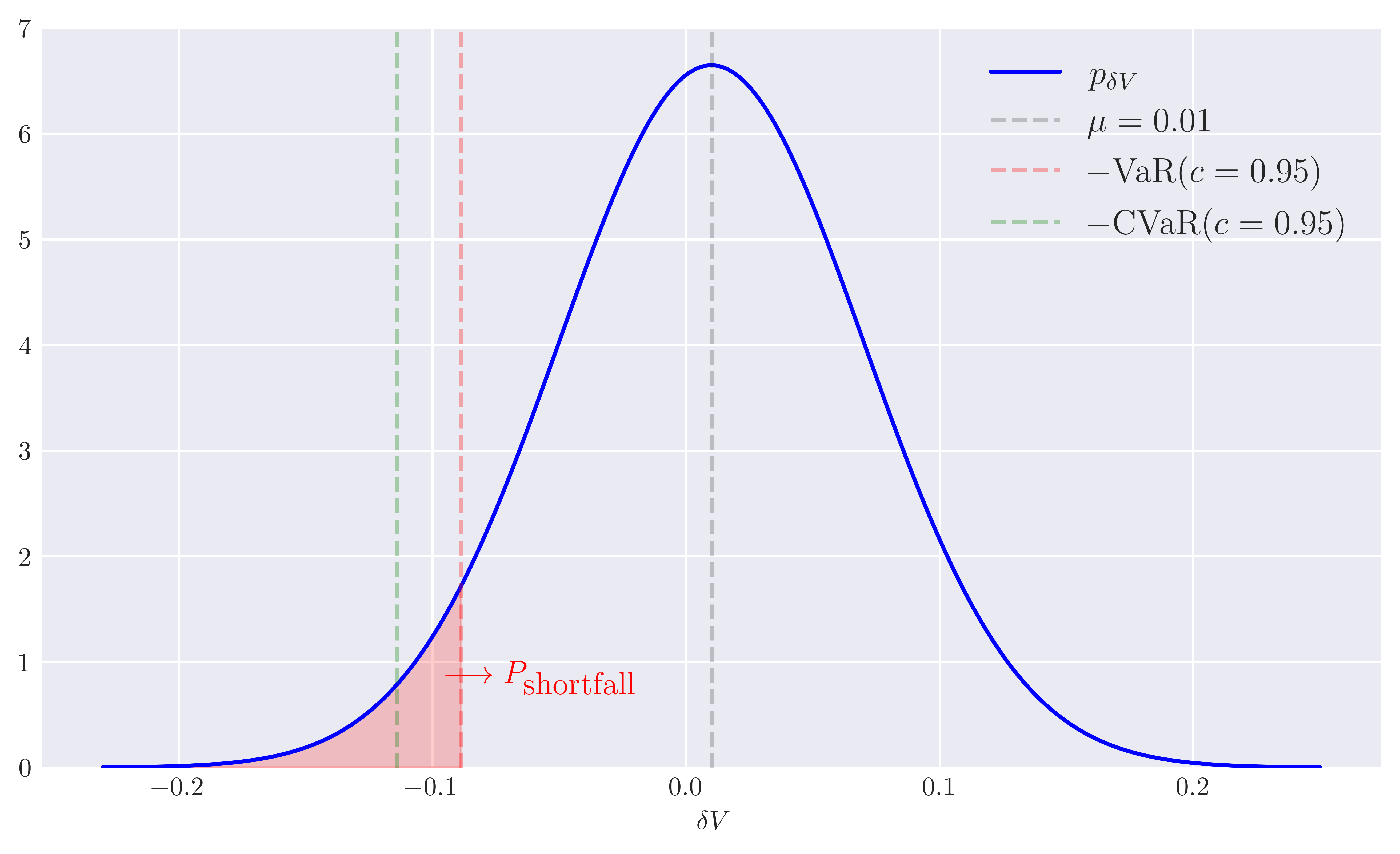Figure 1. VaR and CVaR of a gaussian $\delta V$ distribution with mean $\mu = 0.01$ and standard deviation $\sigma = 0.06$.

Here, we used a confidence interval of 95% ($c = 0.95$). Notice that the shortfall probability is just the area under the curve beyond $1-c$ percentile and of course for the confidence interval we adopt, this area is just given by the cumulative probability distribution \eqref{p_short} between negative values including and beyond $-\textrm{VaR}$:

prob_shortfall = norm.cdf(neg_VaR, mu, sigma)

print(f"Probability of shortfall: {prob_shortfall:.3f}")

Output:

Probability of shortfall: 0.050

The Python code that can be used to reproduce Figure 1 and the result above is given in Appendix A.

References

---

1. “Derivatives and Internal Models: Modern Risk Management”, Hans-Peter Deutsch and Mark W. Beinker .

Appendix A: Code to reproduce Figure 1.

import numpy as np
import matplotlib.pyplot as plt
import matplotlib as mpl
from scipy.stats import norm

mpl.rcParams['text.usetex'] = True

#For inline plotting 
%matplotlib inline                 
%config InlineBackend.figure_format = 'svg'

plt.style.use("seaborn-v0_8-dark")

# Parameters for the normally distributed portfolio change dV
mu = 0.01
sigma = 0.06

# Generate normally distributed data for visualization
dV_interval = np.linspace(mu - 4 * sigma, mu + 4 * sigma, 1000)
dV_normal = norm.pdf(dV_interval, mu, sigma)

# confidence level
c = 0.95

# negative of Value at risk using point percentile function
neg_VaR = norm.ppf(1-c, loc = mu, scale = sigma) 

# CVaR through sampling from a large sample
dV_norm = np.random.normal(loc = mu, scale = sigma, size = (10**6))
neg_CVaR = dV_norm[dV_norm <= neg_VaR].mean()

# Plot the normal distribution, VaR, and CVaR
plt.figure(figsize=(9, 5))
plt.plot(dV_interval, dV_normal, label=r'$p_{\delta V}$', color='blue')

plt.axvline(x=mu, color='black', linestyle='--', alpha = 0.2, label = r'$\mu = 0.01$')

# VaR
plt.axvline(x=neg_VaR, color='red', linestyle='--', alpha = 0.3, label = r'$-\textrm{VaR}(c = 0.95)$') 

# CVaR
plt.axvline(x=neg_CVaR, color='green', linestyle='--', alpha = 0.3, label = r'$-\textrm{CVaR}(c = 0.95)$')

# Fill area under the curve for VaR which gives P_shortfall
plt.fill_between(dV_interval, dV_normal, where=(dV_interval <= neg_VaR), color='red', alpha=0.2)
plt.text(-0.095,0.8, r'$\longrightarrow P_{\textrm{shortfall}}$', color = 'red', fontsize=12) 

plt.xlabel(r'$\delta V$')
plt.ylim(0,7)
plt.legend(fontsize = 13)

plt.grid()