To return or log return?

The notion of “return” is one of the most basic and equally fundamental concept in finance. There are two common definitions that is utilized in the literature: simple returns and log-returns. Arguably, the most of the literature refer to the former when the word “return” is mentioned. Since stock returns are very small, the difference between these two definitions from a purely numerical point of view is small. However, when we consider statistical properties of these variables such as expected values, variances and covariances, significant deviations can arise. In this post, I would like to illustrate the consequences of the misuse of financial returns, in the context of suboptimal portfolio selection and the determination of beta in CAPM.

Return vs log-return

---

We start with the definitions of both returns. Given the price of a security $P_t$ at time $t$, the simple return at time $t$ for an investment on asset $i$ at time $t-1$ (i.e. return for a single discrete time period) is given by

\[\begin{equation}\label{R} R^{(i)}_t = \frac{P^{(i)}_t}{P^{(i)}_{t-1}} - 1. \end{equation}\]

On the other hand, the log-return for the same time period can be defined as

\[\begin{equation}\label{r} r^{(i)}_t = \ln (1 + R^{(i)}_t) = \ln\left(\frac{P^{(i)}_t}{P^{(i)}_{t-1}}\right). \end{equation}\]

Due to appearance of logarithm, the log returns have the appealing property of additivity (along the time axis) for multiple period investments. For example, for an investment between $t = 0$ and $t$, the compounded log-return read as

\[\begin{equation} r^{(i)}_{0:t} = \ln \left(\frac{P^{(i)}_t}{P^{(i)}_0}\right) = \ln \left(\frac{P^{(i)}_t}{P^{(i)}_{t-1}}\frac{P^{(i)}_{t-1}}{P^{(i)}_{t-2}}\dots \frac{P^{(i)}_1}{P^{(i)}_{0}}\right) = r_1 + r_2 + \dots + r_t. \end{equation}\]

When described in terms of the simple returns of assets, the portfolio return (composed of $n$ assets) at time $t$ has a similar (weighted) additivity property

\[\begin{equation}\label{Rp} R^{(p)}_t = \sum_{i = 1}^n w_i R^{(i)}_t, \quad\quad \sum_{i = 1}^n w_i = 1. \end{equation}\]

Recall that Markowitz’s modern portfolio theory utilizes this linear structure in the quest to find efficient portfolios. On the other hand, we know from \eqref{R} and \eqref{r} that simple returns can be related to log-returns as $R = \mathrm{e}^r - 1$ using which with \eqref{Rp} imply the following relationship of portfolio log-returns in terms of the individual asset log-returns:

\[r^{(p)}_t = \ln\left(\sum_{i = 1}^n w_i\, \mathrm{e}^{r^{(i)}_t}\right).\]

Due to non-linearity of this relationship, portfolio managers prefer to work with its linear counterpart \eqref{Rp} using simple returns $R^{(i)}$.

From \eqref{r}, it is clear that the log-returns have support over the entire real line, $r_t \in \mathbb{R}$ while the simple returns defined within an asymmetric range:

\[\begin{equation}\label{Rran} -1 \leq R_t < \infty. \end{equation}\]

This asymmetry does already suggest why simple returns are not a good candidate to exhibit normal distribution as compared to log-returns, which is a natural property of the latter under the random walk hypothesis. Furthermore, for simple returns around zero $R^{(i)}_t \sim 0$, Taylor expansion of eq. \eqref{r} tells us that log-returns can be approximately equivalent to simple returns, $r_t = \ln(1+R_t) \approx R_t$. This approximation is the main source of confusion in many practical implementations involving financial returns.

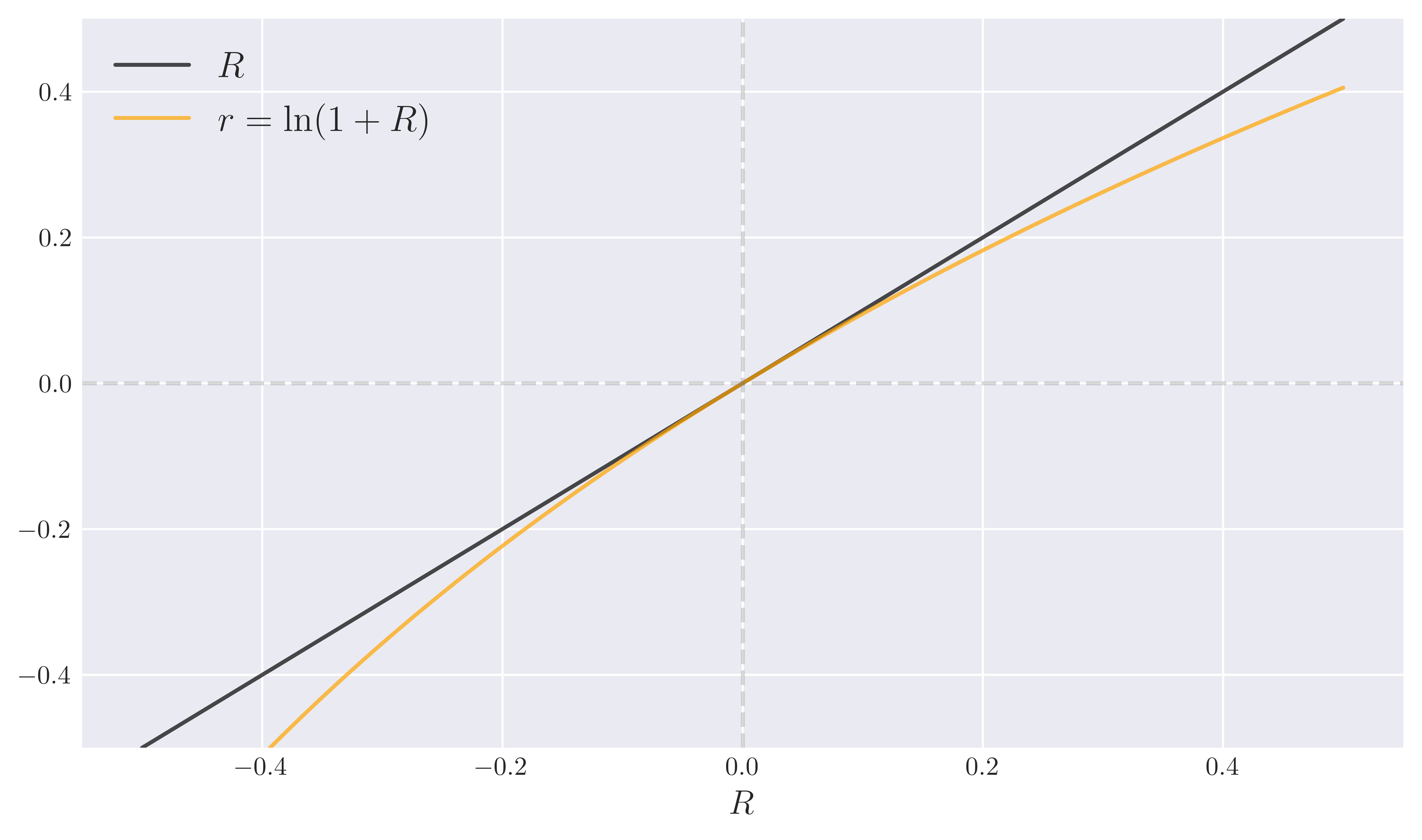Figure 1. Simple returns $R$ vs log returns $r = \ln(1+R)$.

Fig. 1 confirms validity of the $r_t = \ln(1+R_t) \approx R_t$ approximation for $R \sim 0$. On the other hand, for large (simple) returns in absolute value, $|R|\sim \mathcal{O}(1)$, it is clear that the difference between these two notions of return becomes more apparent. It is indeed a well known fact that stock return distributions have tails, exhibiting extreme values of $|R|$ within the range \eqref{Rran}. In this case, we can no longer expect the moments of the simple returns and log-return distributions to match.

As we mentioned earlier, the standard textbook approach of asset pricing models give rise to normally distributed log-returns. In this case, we can compute the moments for the corresponding simple returns. For example, if we take the expected value and variance of log-returns as $\mu_i$ and $\sigma_i^2$ for asset $i$, we have

\[\begin{equation}\label{er} \mu_R = \mathbb{E}[R_i] = \mathbb{E}[\mathrm{e}^{r_i} - 1] = \mathrm{e}^{\mu_i + \sigma_i^2/2} - 1, \end{equation}\]

where we utilized the properties of the moment generating function (MGF) of the normally distributed variable $r_i \sim \mathcal{N}(\mu_i,\sigma_i^2)$ (see Appendix A). Covariance of simple returns of two assets can be also derived in terms of the moments of the log return counterparts as

\[\begin{align} \nonumber \textrm{Cov}(R_i,R_j) &= \mathbb{E}[R_i\, R_j] - \mathbb{E}[R_i]\mathbb{E}[R_j],\\ \nonumber &= \mathbb{E}[(\mathrm{e}^{r_i} - 1)(\mathrm{e}^{r_j} - 1)] - (\mathrm{e}^{\mu_i + \sigma_i^2/2} - 1)(\mathrm{e}^{\mu_j + \sigma_j^2/2} - 1),\\ \nonumber &= \mathbb{E}[\mathrm{e}^{r_i + r_j}] - \mathrm{e}^{\mu_i + \mu_j + (\sigma_i^2 + \sigma_j^2)/2},\\ \label{covsr}&= \mathrm{e}^{\mu_i + \mu_j + (\sigma_i^2 + \sigma_j^2)/2} \left(\mathrm{e}^{\sigma_{ij}} - 1\right) \end{align}\]

following the discussion in the Appendix. Here $\sigma_{ij}$ is the covariance of log returns $\textrm{Cov}(r_i,r_j) =\sigma_{ij}$. Using \eqref{covsr}, variance of individual simple stock returns is given by

\[\begin{equation}\label{varR} \mathbb{V}[R_i] \equiv \textrm{Cov}(R_i,R_i) = \mathrm{e}^{2\mu_i + \sigma_i^2}\left(\mathrm{e}^{\sigma_i^2} - 1\right). \end{equation}\]

The lines above clearly illustrate the potential deviation of different moments of simple returns with respect to log-returns.

Another differentiating concept between two returns appears when annualization of expected returns and (co)-variances is performed. For log returns this is naturally accomplished by following the footsteps of the square root of time rule which is a fundamental property of random walks. Therefore, annualization is most convenient when applied to the different moments of the log-return distribution.

Potential malpractices

---

To illustrate negative consequences of confusing simple returns with log-returns, we will focus on a toy example, discussing in detail how the aforementioned confusion can affect the optimal portfolio selection within Markowitz’s mean-variance analysis.

Portfolio blunder with log-returns:

Let’s assume a fiducial portfolio composed of four risky assets which have (multivariate) normally distributed log returns $\vec{r} = [r_1, r_2, r_3, r_4]^T$ with $\vec{r} \sim \mathcal{N}(\vec{E}, {\bf V})$. We assume the mean log returns and their covariance matrix is given by

\[\begin{equation} \vec{E} = [0.16, 0.14, 0.12, 0.08]^T, \quad\quad {\bf V} = \begin{bmatrix} 0.20 & -0.05 & 0.00 & 0.00 \\ -0.05 & 0.15 & 0.01 & 0.02 \\ 0.00 & 0.01 & 0.10 & 0.00 \\ 0.00 & 0.02 & 0.00 & 0.04 \end{bmatrix}. \end{equation}\]

Adopting the total budget constraint

\[\begin{equation}\label{pc} \sum_{i = 1}^4 w_i = 1, \end{equation}\]

one may tempt to think we have all we need to compute the optimal portfolio allocations based on MPT. However, recall that the inputs for MPT are mean returns and covariances based on simple returns $R$. Utilizing \eqref{er}-\eqref{varR} they are given by

\[\begin{equation} \vec{\mu} = [0.2969, 0.2399, 0.1853, 0.1052]^T, \quad\quad {\bf \Sigma} = \begin{bmatrix} 0.3724 & -0.0784 & 0.0000 & 0.0000 \\ -0.0784 & 0.2488 & 0.0148 & 0.0277 \\ 0.00 & 0.0148 & 0.1478 & 0.0000 \\ 0.00 & 0.0277 & 0.0000 & 0.0498 \end{bmatrix}. \end{equation}\]

Now the standard constrained \eqref{pc} optimization problem can be solved to obtain the efficient portfolios that exhibit the least risk $\sigma_p$ for a given expected return $\mu_p$ within the entire risk-reward spectrum. We perform these calculations in Appendix B. The resulting set of pairs $(\sigma_p, \mu_p)$ that are on the efficient frontier satisfy

\[\begin{equation}\label{eff} \sigma_p(\mu_p) = \sqrt{\frac{A \mu_p^2 - 2 B \mu_p + C}{AC - B^2}}, \quad\quad\quad \textrm{for} \quad \mu_p > B/A, \end{equation}\]

where we defined the following scalar variables in terms of the inverse of the covariance matrix, identity $\vec{1} = [1,1,1,1]^T$ and mean return $\vec{\mu}$ vector as

\[\begin{equation}\label{svs} \vec{1}^T \cdot ({\bf \Sigma}^{-1} \cdot \vec{\mu}) = B, \quad \vec{1}^T \cdot ({\bf \Sigma}^{-1}\cdot \vec{1}) = A, \quad \vec{\mu}^T \cdot ({\bf \Sigma}^{-1}\cdot \vec{\mu}) = C. \end{equation}\]

The condition on the right in eq. \eqref{eff} stems from the fact that $\mu_{p} = B / A$ corresponds to return of the global minimum variance portfolio with the corresponding variance $\sigma_{p}^2(\mu_{p}^{*}) = A^{-1}$. Therefore, $\mu_{p} > B/A$ branch in the risk reward ($\sigma_p - \mu_{p}$) spectrum corresponds to the efficient frontier.

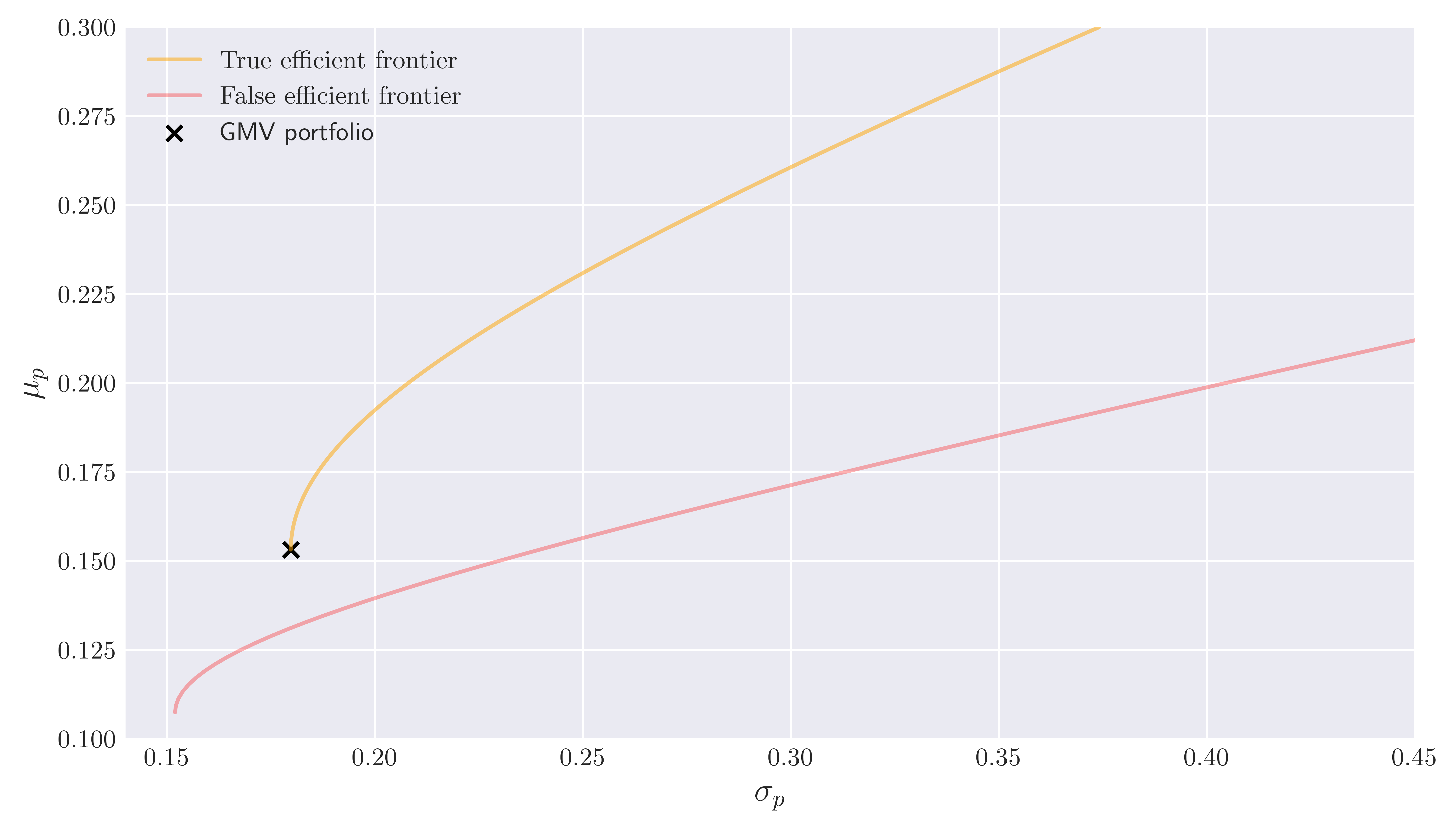Fig. 2. Correct and False efficient frontier via eq. (13).

In Figure 2, we compare the true efficient frontier \eqref{eff} with the one obtained through log returns by replacing ${\bf \Sigma} \to {\bf V}$, $\vec{\mu} \to \vec{E}$ in eqs. \eqref{eff} and \eqref{svs}. We observe that a confusion of the expected values and (co)variances of simple returns with those of the log returns can lead to non-negligibly suboptimal portfolio selection.

References

---

1. “WHY THE RETURN NOTION MATTERS”, GREGOR DORFLEITNER, International Journal of Theoretical and Applied Finance 2003 06:01, 73-86” .

Appendix A: Moment generating function of random normal variables

---

Let $X \sim \mathcal{N}(\mu,\sigma^2)$ be a random normal variable and consider its moment generating function

\[\begin{equation}\label{mgf} M_X (t) = \mathbb{E}[\mathrm{e}^{t X}] = \int_{-\infty}^{\infty} \mathrm{e}^{t x} f_X(x)\, \mathrm{d}x \end{equation}\]

where $f_X$ is the pdf of normal distribution. The expression above is a moment generating function in the sense that we can obtain the expectation values for powers of $X$ by taking derivatives of \eqref{mgf} with respect to $t$ and then by sending $t \to 0$. For example, it is easy to see that $\mathbb{E}[X] = M_X’(0)$. Taking higher derivatives of $M_X$ similar expressions for higher moments can be derived.

Now notice by definition we can write the normal variable as $X = \mu + \sigma Z$ where $Z \sim \mathcal{N}(0,1)$. We can then write the expectation value in \eqref{mgf} as

\[\begin{align} \nonumber \mathbb{E}[\mathrm{e}^{tX}] &= \mathrm{e}^{t \mu} \int_{-\infty}^{\infty} \frac{\mathrm{e}^{(2 t \sigma z - z^2)/2}}{\sqrt{2\pi}} \, \mathrm{dz},\\ \nonumber &= \mathrm{e}^{t\mu + t^2 \sigma^2/ 2} \int_{-\infty}^{\infty} \frac{e^{-y^2/2}}{\sqrt{2\pi}} \mathrm{d}y, \\ \label{mgfr}&= \mathrm{e}^{t\mu + t^2 \sigma^2/ 2} \end{align}\]

where we have completed the exponent inside the integral to a square in the second line defining a new variable of integration via $y = z - t\sigma$. The expression \eqref{mgfr} therefore gives us the expectation of the exponential of a random Gaussian variable as:

\[\begin{equation}\label{mx1} M_X(1) = \mathbb{E}[\mathrm{e}^X] = \mathrm{e}^{\mu + \sigma^2/ 2}. \end{equation}\]

Now consider the sum of two Gaussian random variables $r_i \sim \mathcal{N}(\mu_i,\sigma_i^2)$ and $r_j \sim \mathcal{N}(\mu_j,\sigma_j^2)$ that are correlated as in the case of returns of two stocks. First, the random vector $\vec{r} = (r_i, r_j)^T$ ($i\neq j$) is multivariate normal, $\vec{r} \sim \mathcal{N}(\vec{\mu}, {\bf \Sigma})$ with $\vec{\mu} = (\mu_i,\mu_j)^T$. Then by definition of multivariate distribution, any linear combination of $\vec{r}$ will also be normally distributed. Therefore, consider the special linear combination $r_i + r_j = \vec{1}^T \cdot \vec{r}$ for $\vec{1} = [1,1]^T$ and $(r_i + r_j) \sim \mathcal{N}(\mathbb{E}[r_i + r_j], \mathbb{V}[r_i + r_j])$:

\[\begin{align} \nonumber \mathbb{E}[r_i + r_j] &= \mu_i + \mu_j,\\ \mathbb{V}[r_i + r_j] &= \mathbb{V}[r_i] + \mathbb{V}[r_j] + 2\textrm{Cov}(r_i,r_j). \end{align}\]

On the other hand, since $r_i + r_j$ is normally distributed, it satisfies \eqref{mx1} in an analogous way:

\[\begin{equation} \mathbb{E}[\mathrm{e}^{r_i + r_j}] = \mathrm{e}^{\mathbb{E}[r_i + r_j] + \mathbb{V}[r_i + r_j]/ 2} = \mathrm{e}^{\mu_i + \mu_j + (\sigma_i^2 +\sigma_j^2)/2 + \sigma_{ij}} \end{equation}\]

where we defined the covariance $\textrm{Cov}(r_i,r_j) = \sigma_{ij}$.

Appendix B: Portfolio optimization and the efficient frontier

---

First we focus on the constrained optimization problem of finding portfolio weights $\vec{w}$, which can be formulated as

\[\begin{align} \nonumber \mathop{\textrm{min}}_{\vec{w}}\,\,\sigma_p^2 &= \vec{w}^T \cdot ({\bf \Sigma} \cdot \vec{w}),\\ \textrm{s.t}\,\, \vec{w}^T \cdot \vec{\mu} &= \mu_p\,\, \textrm{and} \,\, \vec{w}^T \cdot \vec{1} = 1. \end{align}\]

We can solve the constrained system using the standard Lagrange multiplier method using the following Lagrangian

\[L\left(\vec{w}, \lambda_1, \lambda_2\right)=\vec{w}^{T} \cdot ({\bf \Sigma} \cdot \vec{w}) +\lambda_1\left(\vec{w}^{T} \cdot \vec{\mu}-\mu_{p}\right) +\lambda_2\left(\vec{w}^{T} \cdot \vec{1}-1\right).\]

Varying the Lagrangian with respect to weight vector gives

\[\begin{equation}\label{solw} \vec{w} = \frac{\lambda_1}{2} {\bf \Sigma}^{-1} \cdot \vec{\mu} + \frac{\lambda_2}{2} {\bf \Sigma}^{-1} \cdot \vec{1}, \end{equation}\]

whereas the variation with respect to Lagrange multipliers $(\lambda_1,\lambda_2)$ give the original constraints trivially. Using these constraints with \eqref{solw}, we can determine $(\lambda_1,\lambda_2)$ solving the following set of equations:

\[\begin{align} \nonumber \vec{w}^{T} \cdot \vec{1} &= 1 \quad \Rightarrow \,\,\,\,\quad \lambda_1 B + \lambda_2 A = 2,\\ \label{lamb}\vec{w}^{T} \cdot \vec{\mu} = \vec{\mu}^T \cdot \vec{w} &= \mu_p \quad \Rightarrow \quad \lambda_1 C + \lambda_2 B = 2\mu_p \end{align}\]

where we defined the following constants in terms of the inverse of the covariance matrix ${\bf \Sigma}^{-1} = ({\bf \Sigma}^T)^{-1} = ({\bf \Sigma}^{-1})^{T}$, mean return $\vec{\mu}$ and the identity vector $\vec{1}$:

\[\vec{1}^T \cdot ({\bf \Sigma}^{-1}\cdot \vec{\mu}) = B, \quad \vec{1}^T \cdot ({\bf \Sigma}^{-1} \cdot \vec{1}) = A, \quad \vec{\mu}^T \cdot ({\bf \Sigma}^{-1}\cdot \vec{\mu}) = C.\]

In terms of these variables the system of equations \eqref{lamb} can be solved to obtain

\[\begin{equation} \lambda_1 = \frac{2(A\mu_p - B)}{AC-B^2},\quad\quad \lambda_2 = \frac{2(C - B\mu_p)}{AC-B^2}. \end{equation}\]

Therefore, the optimal weights \eqref{solw} can be found as

\[\begin{equation} \vec{w}^{*} = {\bf \Sigma}^{-1} \left(\frac{(C - B\mu_p)}{AC-B^2} \vec{1} + \frac{(A\mu_p - B)}{AC-B^2} \vec{\mu} \right). \end{equation}\]

On the other hand, from \eqref{solw} and \eqref{lamb}, the variance of the portfolio returns can be obtained as

\[\begin{align} \nonumber \sigma_p^2 &= \vec{w}^T \cdot ({\bf \Sigma} \cdot \vec{w})\\ \nonumber &= \frac{1}{4} \left(C \lambda_1^2 + 2B\lambda_1\lambda_2 + A \lambda_2^2 \right)\\ \nonumber&= \frac{1}{4} \left(\lambda_1 (\lambda_1 C + \lambda_2 B) + \lambda_2 (\lambda_1 B + \lambda_2 A)\right)\\ \label{ef}&= \frac{1}{AC-B^2} \left(A \mu_p^2 - 2B \mu_p + C\right). \end{align}\]

The relation \eqref{ef} gives the efficient portfolios (frontier) in the $\sigma_p$ and $\mu_p$ plane that have the minimum risk at a desired reward $\mu_p$.