Risk-neutral valuation

In the Black-Scholes option pricing theory, recall that the concepts of risk-neutrality and no-arbitrage appeared to be fundamental in the derivation of option dynamics, as well as the determination of a unique price for a European type contingent claim: i.e. a contract whose pay-off at the expiry is dependent on an event. In fact, the idea of risk-neutrality is so fundamental that it can be taken as the only guide to price European type options. For this purpose, we need to take dive into the world of probabilities contrary to the standard approach based on hedging arguments. We will see that how risk-neutrality provides a model independent framework for pricing derivatives, ensuring no-arbitrage at the same time.

Risk Neutrality

---

To illustrate the main idea, let us consider an example from the world of a horse race bookie whose job is to set the odds for horses and make re-payments to the clients according to these odds while collecting fees about these bets sometime in between. Suppose that we live in a world that only two horses race. Now we consider the following situation:

• Assume that the bookie is quite experienced to be confidently say that the first horse has $20 \%$ chance of winning the race while the second has $80 \%$.
• The population that does not exhibit the experience that the bookie has, places its bets slightly differently by betting a total of $10 k$ USD on the first while putting a total of $50 k$ USD bets on the second horse. This situation reflects the view of the participants in the “market”: for every $60 k$ betted on the race, participants are willing to put $10 k$ on the first and $50 k$ on the second.

If the bookie sets the odds for this race according to the ‘real-world’ probabilities, the second has 4 time more chance of win with respect to the first, so the bookie should reward the every penny invested in the first more due to risk it possess. So she decides odds to be 4-1. This implies that for every 1 USD invested in the first horse, there will be 4 USD profit. Similarly, for every 4 dollars invested in the second horse, on makes one dollar profit. Therefore, if she sets the odds to be 4-1, in the world state where the first horse wins, she pays back a total amount of $(10 + 40) k$ USD for people who bet on the first horse which is $10 k$ less than the total bets $60 k$ she received, making a total of $10 k$ profit. On the other hand, in the world state where the second horse wins, she needs to give back a total amount of $50 k$ plus $12.5 k$, which is $2.5 k$ more than the original amount she received. Therefore, if the second horse wins, she loses $2.5 k$. On average, she does not expect make money from these trades, as her expected profit and loss is given by

\[\mathbb{E}[\textrm{PnL}] = p_1 \times 10.000 - p_2 \times 2500 = 0.2 \times 10.000 - 0.8 \times 2500 = 0, \quad\quad p_1 + p_2 = 1.\]

Although she has zero gains and losses on average, there is a variability of the possible outcomes and the concerning one here is about the possibility that the second horse wins which exhibit a downside risk. Of course, she might collect enough fees from all the bets to cover such downside risks, but this will also show some variability: she will make profit sometimes but also loose some as well for other times. One thing she can do is to reflect those risks to her fees, adjusting it according to the specific “game” to cover her potential losses. However, this would be both impractical (on her side) and of course inefficient for the market (betting industry) because in this case we simply adjust the prices (fee) of the bets according to the risk preferences of the bookie. A more efficient strategy would therefore try to eliminate the uncertainty associated with the PnL outcomes. How can she achieve this?

In fact, she can eliminate her risks by “listening” the market. Instead of focusing on her own analysis of real world probabilities that assigns wining chances for each horse, she can adjust her odds according to the amount people bet on the horses. This would give 5-1 odds as people bet 5 times more money on the second horse than the first. If the first horse wins she needs to pay back a profit of $50 K$ plus the original wager of $10 K$ would completely cover the $60 K$ received initially. If on the other hand the second horse wins, she again pay $10 K$ profit plus the original wager of $50K$, again covering the total initial bets. Therefore, no matter what happens in this two state world, she will be 100 percent sure that she will not lose (or make) money from the transaction itself. Now, she can “carelessly” price the fee for each bet to make money in a risk-free manner which is of course how bookies are operating.

What happened here? From her first attempt to the second, she essentially changed the probabilities that are assigned to each outcome. In the first one, she adjusts her odds according to the real world probabilities while in the second she can be said to adopt risk-neutral probabilities. In particular, by adjusting the odds according to the amount betted on each horse, we can say that the risk-neutral probability that the first horse wins is $\tilde{p}_1 =1/6$ which implies $\tilde{p}_2 = 1 - \tilde{p}_1 = 5/6$ for the second. Mathematically, such a change is referred as a change in the probability measure. The existence of such risk-neutral measures that are “equivalent” to the real world probabilities are essential for the theory of risk-neutral pricing. We will delve into such technicalities once we had developed enough intuition on the main ideas. The simple bookie example we considered here is served for this purpose, giving us a good first idea of how risk-neutral pricing works.

Risk-neutral pricing of Options

---

To illustrate the same idea for European options, we can focus on a similar two state world represented by a single step binomial model. Suppose that the interest rates are zero $r = 0$ and the current stock price at $t = 0$ is 100 which has a probability $p$ of going up to $S_1^{(u)} = 110$ and (with a probability $q = 1-p$) going down to $S_1^{(d)} = 90$ tomorrow. We note that these probabilities reflects the views of the option dealer about how the stock will behave in the future. In this sense they are real world probabilities that are also known to the Market. We would like to know the price of a call option with strike that satisfies $S_1^{(u)} > K = 100 > S_1^{(d)}$ on this underlying. So the option will be certainly exercised in the up-branch (H:head) where it is worth $C_1(H) = S_1(H) - K = 10$ while it has zero value in the down (T:tail) branch $C_1(T)=0$. If the option’s dealer use her views on the behavior of the underlying, she might be tempted to think that the fair price (at $t = 0$) for the option contract would be set by the expected earnings of the client (based on real world probabilities) at the expiry $t = 1$:

\[\begin{equation}\label{cpnf} C_0 = \mathbb{E}[C_1] = p\, C_1(H) + q\, C_1(T), \quad\quad p + q = 1. \end{equation}\]

However, as in the example of the horse race bookie, we are still exposed to risks if we charge the client with \eqref{cpnf} at the inception of the contract. This is because there is a non-zero probability that the option expires in the money, in which case we are obliged to buy the stock from the spot market (at time $t = 1$) to deliver it to the client for a fixed price $K$. This implies that in this world state we will lose an amount equal to the value of the option at the expiry $C_1(H) = S_1(H) - K$ and more importantly this risk is not fully covered with the amount we charge for the option at $t = 0$:

\[C_0 = \mathbb{E}[C_1] = p\, C_1(H) < C_1(H)\]

which holds as the option is worthless in the down-branch $C_1(T) = 0$ and for any real world probability strictly less than unity $p < 1$. A natural question at this point is whether the probability of up can be $p = 1$ ? In fact, it can not because it would imply a simple arbitrage opportunity: one can borrow money at the risk-free rate ($r = 0$) and use it to immediately buy the stock at $t = 0$, tomorrow our asset will worth more than the loan amount we owe to the bank, implying a riskless profit. Of course, for $p < 1$ there will be times that we will make money from selling to contract at is has a non-zero chance for the option to end out-of-money. The point is that there will be a variability of the outcomes on our end.

As a market maker, we do not like to take such risks, so it would not be to our advantage to look at the future world states using the real world probabilities. To protect ourselves from the probability of stock going up tomorrow, we can hedge our position in the call option by buying a certain $\Delta_0$ amount of the underlying at $t = 0$. Now we hold a portfolio that takes two potential values tomorrow, $V^{(p)}_1(H)$ and $V^{(p)}_1(T)$. Our goal is now to remove the risk associated with the portfolio. We can achieve this by demanding our portfolio to have the same value, independent of all world states tomorrow. This determines the amount we need to buy the stock:

\[\begin{equation}\label{delta} \Delta_0 S_1(H) - C_1(H) = \Delta_0 S_1(T) - C_1(T), \quad \Rightarrow \quad \Delta_0 = \frac{C_1(H) - C_1(T)}{S_1(H)-S_1(T)}. \end{equation}\]

Plugging the numbers, $C_1(H) = 10$, $C_1(T) = 0$, $S_1(H) = 110$, $S_1(T) = 90$, gives $\Delta_0 = 1/2$ and our portfolio is worth $V_1 = 45$ for both states $(T,H)$ of the world tomorrow. This simply means that, the portfolio value agrees with 45 riskless bonds in every state of the world tomorrow and since we assume zero interest rates $r = 0$, it must have the same value of 45 riskless bounds today! This is consistent with the no-arbitrage principle based on the monotonicity theorem. Another way of saying this is that since the portfolio is risk-free, it should evolve with the risk-free rate from $t = 0$ to $t = 1$. Since the risk-free rate is assumed to be zero, portfolio value tomorrow is equal to portfolio value today:

\[\begin{equation} V_1^{(p)} = V_0^{(p)}, \quad \Longrightarrow \quad C_0 = \Delta_0 (S_0 - S_1(H)) + C_1(H). \end{equation}\]

Re-arranging terms using the general expression for $\Delta_0$ \eqref{delta}, the price of the call option can be cast into an expectation over its possible values at time $t = 1$:

\[\begin{equation}\label{rnp} C_0 = \tilde{p}\, C_1(H) + \tilde{q}\, C_1(T), \quad\quad \tilde{p} \equiv \frac{S_0 - S_1(T)}{S_1(H) - S_1(T)}, \quad \tilde{q} \equiv 1 - \tilde{p}. \end{equation}\]

Notice that $\tilde{p}$ and $\tilde{q}$ have nothing to do with the real world probabilities, but they are in fact probabilities as they satisfy $0 < \tilde{p},\tilde{q} < 1$ and $\tilde{p} + \tilde{q} = 1$. By the nature of the risk-neutral approach that the option dealer undertake, they are called the risk-neutral probabilities. This is the most logical way to derive the fair price an option like contract, as it sets the pricing method free from the riskiness of the world by not taking such uncertainties into account in the pricing process. Plugging the numbers in \eqref{rnp} gives a special risk-neutral probabilities in our example: $\tilde{p},\tilde{q} = 1/2$ so that under the risk-neutral probability measure, it is equally likely for the stock to go up or down. Note that in essence, dealer has changed the probability measure in her binomial tree model from the real world $\mathbb{P}$ to a risk-neutral one typically denoted by $\mathbb{Q}$. The risk neutral price of the option (in a world with no risk-free interest rates) is thus can be written as

\[\begin{equation} \mathbb{E}_\mathbb{Q}[C_1] = C_0 = \tilde{p} C_1(H) + \tilde{q}\, 0 \end{equation}\]

which gives $C_0 = 5$ for our example. One might wonder what is the expected value of the stock price tomorrow? In this risk-neutral world it is given by

\[\begin{equation} \mathbb{E}_{\mathbb{Q}}[S_1] = \tilde{p} S_1(H) + \tilde{q} S_1(T) = 0.5 \times 110 + 0.5 \times 90 = 100 = S_0 \end{equation}\]

which is the same as today’s price $S_0 = 100$ and since we assume interest rates to be zero, this is the same as a risk-free bond of value 100 today. This implies that in the world described by the probability measure $Q$, the investors are risk-neutral in the sense that they do not require an additional reward for the riskiness of the stock over a risk-free bond. Furthermore, in this world, every market instrument’s value today is equal to its risk-neutral expected value tomorrow:

\[\begin{equation}\label{sms} \mathbb{E}_{\mathbb{Q}}[C_1] = C_0, \quad \mathbb{E}_{\mathbb{Q}}[S_1] = S_0, \quad \mathbb{E}_{\mathbb{Q}}[B_1] = B_0. \end{equation}\]

In this world with no interest rates, the random processes describing these assets are therefore martingales which is a favorite topic of all mathematicians interested in finance. More formally, a (discrete) martingale process $X_i$ satisfies

\[\begin{equation} \mathbb{E}[X_r | {F}_k] = X_k \end{equation}\]

where $r$ denotes a time later than $k$, i.e. $r > k$ and $F_t$ denotes the space of events determined at time $t$. The set of these spaces is called the filtration of information. Clearly, we have $F_{t_1} \subset F_{t_2}$ for $t_1 < t_2$. We will learn more about the properties of martingales later on when we extend our tree model to make it more realistic, e.g. with more time steps and including a non-trivial risk-free rate of borrowing money $r \neq 0$.

I would like to finish this section by emphasizing an important statement made by the eq. \eqref{sms}. Recall that since the expectation is linear, the martingale condition under the risk neutral probability will be valid for any portfolio that is a linear combination of the assets in \eqref{sms}. This implies that if a portfolio has zero value today, it must have expected value of zero tomorrow. Such a portfolio is a no-arbitrage portfolio as there is a non-vanishing probability of negative value for such a portfolio.

This argument shows that if the instruments are priced according to the risk-neutral / martingale measure using its expectation under that measure, then there can be no-arbitrage! Risk-neutrality directly ensured no-arbitrage which is something we expect from an efficient market.

Putting back the interest rates in

Before considering more complicated trees, let’s get ourselves out of the world that does not offer risk-free interest rates. Now we assume that the continuous compounding interest rate is $r > 0$ so that if at time zero the riskless bond is worth 1, it will become $\mathrm{e}^{r \delta t}$ at time $\delta t$ corresponding to a unit discrete time interval. Taking a single step binomial tree as a basis for more complicated trees, the stock prices tomorrow now need to satisfy a relation with respect to the risk-free growth rate of the stock. In particular, we have

\[\begin{equation}\label{na} S_{\delta t}(T) < S_0\, \mathrm{e}^{r \delta t} < S_{\delta t}(H) \end{equation}\]

because otherwise we have arbitrages opportunities to make risk-free profit. What are the risk-free probabilities in this case? Now we have the interest rate, the expected value of the stock at time $\delta t$ should be equal to the asset’s value invested at the risk-free growth rate:

\[\begin{equation} \mathbb{E}_{Q}[S_{\delta t}] = \tilde{p} S_{\delta t}(H) + (1-\tilde{p}) S_{\delta t}(T) = S_0 \, \mathrm{e}^{r\delta t}, \end{equation}\]

which gives

\[\begin{equation} \tilde{p} = \frac{S_0\,\mathrm{e}^{r\delta t} - S_{\delta t}(T)}{S_{\delta t}(H)- S_{\delta t}(T)}. \end{equation}\]

Notice the slight modification that the interest rate bring with respect to the eq. \eqref{rnp}. Furthermore, due to the no-arbitrage constraint \eqref{na}, the risk neutral probability satisfies $0 < \tilde{p} < 1$ as expected from a probability measure that does not like arbitrage.

With the introduction of a non-trivial risk-free rate, every portfolio does not have an expectation value tomorrow that is equal to today’s value, instead its expectation should be equal to the portfolio’s value as if invested at the risk-free growth rate at $t = 0$. Equivalently, the asset’s/portfolio’s expectation discounted by the riskless bond should be equal to today’s value:

\[\begin{equation} \mathbb{E}_{\mathbb{Q}}\left[\frac{A_{\delta t}}{B_{\delta t}}\right] = \frac{A_0}{B_0}. \end{equation}\]

For every asset $A$ it is therefore the process $A_i / B_i$ (in the discrete sense) act as a martingale under the risk-neutral probability measure. Therefore, for a call (or put) option, its risk-neutral pricing in the single step binomial model implies

\[\begin{align} \nonumber C_0 &= \mathrm{e}^{-r \delta t} \mathbb{E}_{\mathbb{Q}}[C_{\delta t}],\\ & = \mathrm{e}^{-r \delta t} \left(\tilde{p}\, f(S_{\delta t}) + (1-\tilde{p})\, f(S_{\delta t})\right) \end{align}\]

where we indicated the options value at $\delta t$ in terms of a general pay-off function $f$ that depends on the stock value at both world states to purposefully emphasize that the same formula applies to any European contingent claim whose value is determined at maturity.

Considering multiple time steps

To be able to converge closer to the real world, we may add more time steps to our binomial tree. For this purpose, let’s consider the 4-step tree showin in Figure 1.

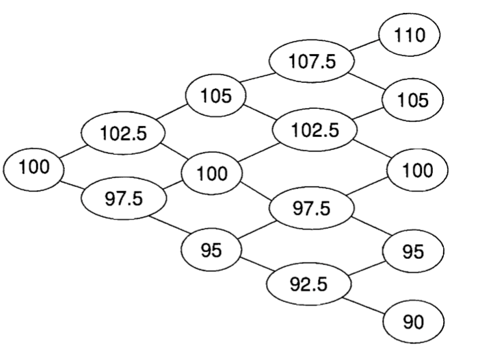Figure 1. 4-step binomial tree for the Stock prices between time $t = 0$ until the maturity of the option at $t = T$.

We consider splitting the equally spaced time increments of $\delta t = T/n$ where $n$ is the number of time-steps. Since we assume the bonds evolve deterministically with an initial value of $B_0 = 1$ at $t = 0$, we have $B_1 = \mathrm{e}^{r T /4}$, $B_2 = \mathrm{e}^{2 r T /4}$ and so on for a risk-free compounding interest rate of $r$. Assuming that the probabilities coming out of each node on the tree are the risk neutral probabilities, we can gain more insight on some properties of the martingales. Now consistent with our previous explorations, in the presence of non-trivial risk-free interest rate, these probabilities can be characterized as

\[\begin{equation}\label{rnpt} \tilde{p}_{N,i} = \frac{S_{N,i-1}\, \mathrm{e}^{r T /4} - S^{(-)}_{N,i}}{S^{(+)}_{N,i} - S^{(-)}_{N,i}} = \frac{S_{N,i-1}\, \mathrm{e}^{r T /4} - S^{(-)}_{N,i}}{5}, \end{equation}\]

where $N$ denotes the node the process currently at as the information reveals to us, e.g. through a successive coin tosses whereas $i$ labels the time index. Notice that for each node $N$ in the tree, the difference between the up and down branch in the next time step is always $S^{(+)}_{i} - S^{(-)}_i = 5$. By construction, this ensures that $S/B$ is a martingale. Let’s have a look at this process as the information unravels. At time step one, the expected value of the $S_1/B_1$ contingent on the Filtration implied by $F_0$ is given by:

\[\begin{equation}\label{s1m} \mathbb{E}_{\mathbb{Q}}\left[\frac{S_1}{B_1} \bigg| F_0\right] = \frac{S_0}{B_0}. \end{equation}\]

Note that at time zero we actually have no information about the process itself and the expectation above is equivalent to standard expectation under risk neutral measure:

\[\mathbb{E}_{\mathbb{Q}}[X_1 | F_0] = \mathbb{E}_{\mathbb{Q}}[X_1] = X_0.\]

Noting $B_1 = \mathrm{e}^{r T/4}$ and $B_0 = 1$, eq. \eqref{s1m} reads

\[\begin{align} \nonumber S_0 &= \mathrm{e}^{-r T /4}\,\mathbb{E}_{\mathbb{Q}}\left[{S_1}\right],\\ \nonumber 100 &= \mathrm{e}^{-r T /4} \left[\tilde{p}_{0,1}\cdot 102.5 + (1 - \tilde{p}_{0,1})\cdot 97.5\right],\\ \nonumber 100 &= \mathrm{e}^{-r T /4} \left[5 \tilde{p}_{0,1} + 97.5\right] \end{align}\]

which is satisfied if the risk-neutral probability of an up move from the zeroth node satisfies eq. \eqref{rnpt}:

\[\tilde{p}_{0,1} = \frac{100 \cdot \mathrm{e}^{r T /4} - 97.5}{5}.\]

The second time step in our process is much more interesting, applying the martingale condition to $S/B$ we have

\[\begin{equation}\label{s2m} \mathbb{E}_{\mathbb{Q}}\left[\frac{S_2}{B_2} \bigg| F_1\right] = \frac{S_1}{B_1}. \end{equation}\]

Now unlike the stock price ($S_0$) at the starting node, the variable on the right-hand side is also random taking two possible values. This fact renders implication of the filtration $F_1$ more interesting. Recall that, $F_1$ represents the space of events determined at the first time step. In other words, it revels us the set of paths that are possible in our 4-step coin toss experiment conditioned on the outcome of the first toss. For example, if the first toss is heads, the following space of events (paths) will be revealed to us an information:

\[\begin{equation} \nonumber A_H = \{HHHH, HHHT, HHTT, HTTT, HHTH, HTHH, HTTH, HTHT\} \in F_1. \end{equation}\]

On the other hand if the outcome of the first toss is tails, we have

\[\begin{equation} \nonumber A_T = \{TTTT, TTTH, TTHH, THHH, TTHT, THTT, THTH, THHT\} \in F_1. \end{equation}\]

as the space of possible events. Notice that in our tree, the union of these spaces $A_T \cup A_H$ determines the set of all distinct paths that determines the stock price at the final time step.

For the expectation value we are after in \eqref{s2m}, filtration therefore gives us the expected value of the discounted price in the second time step given that we have the information that we are either in the head branch ($S^{(+)}_1/B_1$) or the tail branch ($S^{(-)}_1/B_1$). The expression \eqref{s2m} nicely captures this randomness of the $S_1/B_1$ through the filtration $F_1$. Considering our tree, eq. \eqref{s2m} simply tells us that with the information available to us at the first time step the risk neutral expected value of $S_2/B_2$ is nothing but $S^{(\pm)}_1/B_1$. This just means that all I can expect from the next time step is just what we already have/have revealed:

\[\begin{align} \nonumber \frac{S_1}{B_1} &= \mathbb{E}_{\mathbb{Q}}\left[\frac{S_2}{B_2} \bigg| F_1\right],\\ \mathrm{e}^{-r T/4} \left\{\begin{array}{lr} 102.5 \\ 97.5 \end{array}\right\} &= \left\{\begin{array}{lr} 5\tilde{p}_{1^{+},2} + 100 \\ 5\tilde{p}_{1^{-},2} + 95 \end{array}\right\} \end{align}\]

which is of course satisfied for our tree given that probabilities are defined by \eqref{rnpt}.

Something even more interesting occurs if we take the expectation of \eqref{s2m} conditioned on the filtration $F_0$ (e.g no information):

\[\begin{equation} \mathbb{E}_{\mathbb{Q}}\left[\mathbb{E}_{\mathbb{Q}}\left[\frac{S_2}{B_2} \bigg| F_1\right]\bigg | F_0\right] = \mathbb{E}_{\mathbb{Q}}\left[\frac{S_1}{B_1} \bigg| F_0\right] = \frac{S_0}{B_0}. \end{equation}\]

Notice that on the left-hand side, the random variable implied by the

\[\mathbb{E}_{\mathbb{Q}}\left[\frac{S_2}{B_2} \bigg| F_1\right]\]

is conditioned on no information $F_0$ (or more restricted information as compared to the one implied by $F_1$) in the outermost expectation. As a result the total expectation is equivalent to expectation of the random variable itself:

\[\begin{equation} \mathbb{E}_{\mathbb{Q}}\left[\mathbb{E}_{\mathbb{Q}}\left[\frac{S_2}{B_2} \bigg| F_1\right]\bigg | F_0\right] = \mathbb{E}_{\mathbb{Q}}\left[\frac{S_2}{B_2} \bigg| F_0\right] = \mathbb{E}_{\mathbb{Q}}\left[\frac{S_2}{B_2} \right] = \frac{S_0}{B_0}. \end{equation}\]

Here nothing but the Tower Law is at play: which states that if $X_t$ is a discrete martingale, we have

\(\begin{equation} \mathbb{E}\left[\mathbb{E}[X_{n+m} | F_{n + m -1}] | F_n \right] = \mathbb{E}[X_{n+m} | F_n] = X_n. \end{equation}\) By induction, we thus arrive at

\[\begin{equation} \mathbb{E}_{\mathbb{Q}}\left[\frac{S_T}{B_T} \right] = \frac{S_0}{B_0} \quad \Longrightarrow \quad \mathbb{E}_{\mathbb{Q}}\left[{S_T}\right] = S_0 \mathrm{e}^{r T}. \end{equation}\]

In the world of risk neutral probabilities, we can apply the same arguments by tracking the discounted value of a call/put option on the tree. Since we know its value at the maturity $C_T = \textrm{max}(S_T - K, 0) = (S_T - K)_{+}$, we have

\[\begin{equation}\label{rnpg} \mathbb{E}_{\mathbb{Q}}\left[\frac{C_T}{B_T}\right] = \frac{C_0}{B_0} \quad \Longrightarrow \quad C_0 = \mathrm{e}^{-r T} \mathbb{E}_{\mathbb{Q}}[(S_T - K)_{+}]. \end{equation}\]

It is important emphasize that we can interpret this result in a model independent manner. All it tells us that we can obtain the fair price of an option if we know the probability distribution function of the stock price at the maturity of the contract:

\[\begin{equation}\label{corn} C_0 = e^{-rT} \int_{K}^{\infty} (S_T - K) f_{\mathbb{Q}}(S_T) \mathrm{d}S_T. \end{equation}\]

In fact, the second derivative of this expression w.r.t the strike directly allow us to reach at the pdf:

\[\begin{equation} \frac{\partial^2 C_0(K)}{\partial K^2} = f_{\mathbb{Q}}(K). \end{equation}\]

This would imply that from the observed option prices we can derive the risk-neutral probability density function of the stock price. This is where the model independence of the risk-neutral pricing method comes into play. In this sense, risk-neutral pricing provides a robust framework that has some practical implications.

Returning to our binomial tree model, we can re-derive the Black-Scholes price of options by making a few improvements to our model. First, instead of modelling each coin toss in terms of the Stock price, we should model the log-price changes at each time step as a Bernoulli trial (scaled with constant volatility). Then we can make our tree finer and finer by taking the number of steps to infinity $n \to \infty$. By CLT, the distribution of the log stock prices will then converge to normal distribution under the risk neutral measure similar to what is implied by the GBM process:

\[\begin{equation} \ln S_T - \ln S_0 \sim N((r-\sigma^2/2)T, \sigma^2 T). \end{equation}\]

We can then simply compute price of call option using \eqref{rnpg} and \eqref{corn}:

\[\begin{align} \nonumber C_0 &= e^{-r T} \mathbb{E}_{Q} \left[(\mathrm{e}^{\ln S_0 + (r-\sigma^2/2)T + \sigma \sqrt{T} N(0,1)} - K)_{+}\right],\\ &= e^{-r T} \left(S_0 \mathrm{e}^{(r-\sigma^2/2)T}\int_{-d_2}^{\infty} \mathrm{e}^{\sigma^2 T /2} \mathrm{e}^{-(z - \sigma \sqrt{T})^2/2} \mathrm{d}z - K \int_{-d_2}^{\infty} \mathrm{e}^{-z^2/2} \mathrm{d}z \right), \end{align}\]

where we completed the integrand of the first integral into a square and defined

\[d_2 = \frac{\ln (S_0/K) + (r - \sigma^2/2)T}{\sigma \sqrt{T}}.\]

The integral in the second terms just gives cumulative probability that the option will end in the money: $N(d_2)$ whereas the integral in the first term can be shown to yield $N(d_2 + \sigma \sqrt{T})$ by a change of variable $z’ = z - \sigma \sqrt{T}$. Leaving us with the Black-Scholes price of a call option:

\[\begin{equation} C_0 = S_0 N(d_2 + \sigma \sqrt{T}) - K\, \mathrm{e}^{-r T} N(d_2). \end{equation}\]

Conclusions

---

Risk-neutral pricing method provides a practical framework for pricing European type derivative contracts. While we were exploring this concept, we touched upon many useful mathematical structures that it relies on. Notably, we saw that how the introduction of martingales simplifies the derivation of option pricing. While we applied it to a certain model of options whose underlying evolves in a binomial-tree, risk-neutral pricing has a model independent characteristic that can in principle be applied to any European contingent claim as long as we have an accurate estimate on the probability distribution of the underlying asset (see eq. \eqref{corn}). In another post, I would like dive deeper into the implications of this last statement, especially on how we can in practice derive this distribution by the observation of options that have high liquidity in the markets.

References

---

1. Topics in Mathematics with Applications in Finance Lectures, by Dr. Peter Kempthorne, Dr. Choongbum Lee, Dr. Vasily Strela, Dr. Jake Xia, MIT, Sloan School of Management, 2013.

2. “The concepts and practice of mathematical finance”, Second Edition, Mark S. Joshi.

3. Probability and Stochastic Calculus for Finance Lecture, Lecture on Martingales, Indian Institute of Technology Kanpur.