Modern Porfolio Theory (MPT)
I explore the concept of diversification as an investment strategy its mathematical foundations set by the so called Modern Portfolio Theory.
Anyone who had a glimpse of interest in investing in the financial markets may have heard that diversification matters. But what does diversification actually imply? Intuitively, it refers to investing in assets that are diverse in nature in order to diminish the chances of losing all our money at once. In this post, I would like to gain more insight into these matters by formalizing this intuition through a mathematical framework called Modern Portfolio Theory (also called mean-variance analysis) developed by Harry Markowitz in 1952.
As we will see the central idea behind this framework is that the risk involved in an investment portfolio is not just depend on the performance of individual assets but the correlation between those assets (or asset performances). As a result, MPT suggests that it would be wiser to compile portfolios based on risk-adjusted return rather than constructing portfolios based on simply maximizing returns.
What is a Portfolio, and why is it useful?
Putting it in simple terms, a portfolio is a collection of a number of $n$ securities that are defined with specified weights that usually sum up to unity:
\[\begin{equation}\label{w} \vec{w} = \left[ w_1, w_2, \dots, w_n \right]^T, \quad\quad \sum_{i = 1}^n w_i = 1. \end{equation}\]Here, weights simply characterize the proportion of the $i$th asset in the portfolio. For example, if $N_i$ is the number of shares we have for an asset priced at $P_i$, then $w_i$ reflects the ratio between money we invested in that asset with respect to the total value of the portfolio:
\[\begin{equation}\label{iw} w_i = \frac{N_i\, P_i}{\sum_{j = 1}^{n} N_j P_j} \end{equation}\]Number of shares $N \in \mathbb{Z}$ can be positive, zero, as well as negative. Therefore, weights could be negative as well: for example we can short sell (betting on the stock price will go down) a stock we don’t have by borrowing that stock from someone else. Considering a two asset portfolio, the weight of the other asset should be greater than one in this case so as the satisfy the constraint in eq. \eqref{w}. This implies a leveraged transaction, i.e. we are buying more than we have by using the money we obtain from selling the stock we borrowed (short selling). There is also the possibility the weights sum up to zero, corresponding to a dollar-neutral portfolio where the portfolio holds long and short positions with an equal amount in capital. Many hedge fund strategies are based on such portfolios. However, I will not cover this possibility and stick with our good old constraint in eq. \eqref{w}. In summary, we assume that portfolio weights characterize all the relevant information about our investment portfolio.
To illustrate this, consider that we have an investment portfolio composed of 200 shares of asset A with a 50 USD price/share, 1000 shares of asset B with a 30 USD price/share and 600 shares of asset C with a 100 USD price/share. Instead of using these quantities, we can completely characterize this portfolio by weights \eqref{iw} with the help of the Table below
| Asset | Shares | Price/Share | Investment [$] | $w_i$ |
|---|---|---|---|---|
| A | 200 | 50$ | 10.000$ | 0.1 |
| B | 1000 | 30$ | 30.000$ | 0.3 |
| C | 600 | 100$ | 60.000$ | 0.6 |
Thus, the proportion of asset A in our portfolio would be 10 % while B would take up 30 % and the biggest slice would go to asset C with 60 %. Note that as envisioned by the eq. \eqref{iw}, portfolio weights just measure the proportion of dollar investment (4th column) for the $i$th asset with respect to the total portfolio value of 100.000$.
Another more complicated example would be the case when your broker inform you about the possibility of investing on margin, which implies that we can support the same portfolio by only keeping some proportion of the total portfolio amount in the account while borrowing rest from a bank/broker or by short selling a riskless security, e.g. riskless bonds:
| Asset | Shares | Price/Share | Investment [$] | $w_i$ |
|---|---|---|---|---|
| A | 200 | 50$ | 10.000$ | 0.2 |
| B | 1000 | 30$ | 30.000$ | 0.6 |
| C | 600 | 100$ | 60.000$ | 1.2 |
| Riskless Bonds | -50.000 | 1$ | -50.000$ | -1. |
In this case we were allowed the leverage our long positions (equities), as the total investment we made (the sum of all rows corresponding to Investment column), or the total amount we need to keep in our account is 50.000$. In other words, using bonds we are levering up equity positions.
Why do we care about Portfolios?
We already made an earlier statement about the usefulness of portfolios as they enable us to combine assets with different downside risks to potentially reduce losses. However, there is another approach championed by people like Warren Buffet who criticized this diversification concept by stating that you can put all your eggs in one basked and then watch that basket really carefully. For an experienced investor like Warren Buffet this approach may work however for an average investor, information about a certain stock or company is not immediately available, often leaving him/her with a lack of informed decision process on how to pick the right basket. The central idea behind MPT is simply to develop a relatively systematic approach (that can appeal to most of us) to making informed investment decisions by accepting the fact that most of the investors are not alike Warren Buffet and not interested becoming like him either.
Therefore, assuming we don’t know how to pick the best stock, portfolio theory aims to find a responsible and attractive way of investing that has some economic logic brewed by the fundamental notions’ mathematics/statistics.
Now an important question in this line of reasoning is what are the characteristics of a “good” portfolio? We can describe a desirable portfolio as a one with high expected reward but low risk, where “reward” is defined as overall portfolio return and “risk” is defined as the volatility (variance or standard deviation) of that return. This statement relies on the assumption that investors like to have portfolios that have higher mean returns and low standard deviation of returns.
Given this definition of a desirable portfolio, an important question is how do we choose asset weights ${\bf w}$ to optimize the risk-reward characteristics of the overall portfolio? The answer to this question is main aim of the so called mean-variance analysis/optimization that I will cover later on in this post.
Risk reduction by diversification
Before we dive into mean-variance analysis to infer the optimal weights $\vec{w}$ of a portfolio, it is useful to define the risk and reward measures of a portfolio. For this purpose, it is convenient to take a bottom up approach by first considering the parameters that quantifies the risk and reward associated with individual assets that make up a portfolio.
In the absence of an accurate forecasting mechanism, all we can do is the look at the distribution of past returns $r_i$ of the $i$th asset. We define its expected (mean) value and the variance as
\[\begin{align} \nonumber \mathbb{E}[r_i] &\equiv \mu_i,\\ \label{msa}\mathbb{V}[r_i] &= \mathbb{E}[(r_i - \mu_i)^2] \equiv \sigma^2_i. \end{align}\]Next we define the portfolio return as the weighted sum of individual asset returns as
\[\begin{equation}\label{Rp} R_p = w_1 r_1 + w_2 r_2 + \dots + w_n r_n = \sum_{i = 1}^{n} w_i\,r_i = \vec{w}^T \cdot \vec{r}\, , \end{equation}\]where we defined return vector of our asset universe $\vec{r} = [r_1,r_2,\dots,r_n]^T$. By the linearity of the expectation value, the expected portfolio return is simply given by
\[\begin{align} \nonumber \mathbb{E}[R_p] &\equiv \mu_p \\ \nonumber &= \mathbb{E}\left[\sum_{i = 1}^n w_i r_i\right],\\ \nonumber &= \sum_{i = 1}^n w_i \mathbb{E}[r_i] , \\ \label{mup} &= \vec{w}^T \cdot \vec{\mu} \end{align}\]On the other hand, the variance of portfolio returns can be defined as
\[\begin{align} \nonumber \mathbb{V}[R_p] &\equiv \sigma_p^2, \\ \nonumber &= \mathbb{E}\left[\left(R_p-\mu_p\right)^2\right],\\ \nonumber &= \mathbb{E}\Bigg[\left(\sum_{i = 1}^n w_i (r_i - \mu_i)\right)^2\Bigg],\\ \nonumber &= \mathbb{E}\Bigg[\left(\sum_{i = 1}^n w_i (r_i - \mu_i)\right)\left(\sum_{j = 1}^n w_j (r_j - \mu_j)\right)\Bigg], \\ \label{varp} &= \sum_{i = 1}^{n} \sum_{j = 1}^{n} w_i w_j \, \mathbb{E}\left[(r_i - \mu_i)(r_j - \mu_j)\right] \end{align}\]where we utilized \eqref{Rp} and \eqref{mup} in passing from second to third line and the linearity of the expectation value when we move from fourth to the last line. The quantity on the right can be defined as the covariance matrix of returns
\[\begin{equation}\label{cov} \Sigma_{ij} \equiv \mathbb{E}\left[(r_i - \mu_i)(r_j - \mu_j)\right] = \mathrm{Cov}[r_i,r_j] \end{equation}\]As the variance of portfolio returns is a scalar quantity, the double sum is invariant under the exchange of dummy indices $i \leftrightarrow j$ in \eqref{varp}. This implies that covariance matrix is also symmetric under this exchange which can be seen easily using the Einstein summation notation:
\[\begin{equation}\label{varp2} \sigma_p^2 = w_i \, w_j \, \Sigma_{ij} = w_j\, w_i \, \Sigma_{ji} = w_i\, w_j \, \Sigma_{ji},\quad \Rightarrow \quad \Sigma_{ij} = \Sigma_{ji} \end{equation}\]where summation over the dummy indices $i,j$ is implied. For a number of $n$ assets in our portfolio, there are a total of $n^2$ components in the covariance matrix. By definition (see eqs. \eqref{cov} and \eqref{msa}), $n$ of these components corresponding to the diagonal $i = j$, is just the variance squared of the asset returns
\[\begin{equation} \Sigma_{ii} = \textrm{Cov}[r_i,r_i] = \delta_{ij}\, \sigma_i \sigma_j = \sigma_i^2 \end{equation}\]This leaves us with $n^2 - n$ non-diagonal components with $i \neq j$. Furthermore, within these non-diagonal components only $(n^2 - n)/2$ number of them are independent due to symmetry property of $\Sigma_{ij}$.
Now recall that the concept of covariance is tightly related to the correlation between two random variables. In fact correlation matrix can be defined as the scaled version of the covariance matrix:
\[\begin{equation}\label{corr} \rho_{ij} = \frac{\textrm{Cov}[r_i,r_j]}{\sigma_i \sigma_j} = \frac{\Sigma_{ij}}{\sigma_i \sigma_j} \quad\quad -1 \leq \rho_{ij} \leq 1, \end{equation}\]where the scaling is performed using the standard deviation of individual assets within the portfolio. Utilizing \eqref{corr} enables us to write the portfolio variance in a compact way that can account for both the diagonal and cross terms that appear in eq. \eqref{varp2}:
\[\begin{align} \nonumber \sigma_p^2 &= w_i\, w_j \Sigma_{ij}\\ \nonumber &= \vec{w}^T \cdot (\, {\bf \Sigma}\cdot \vec{w})\\ \label{varpf} &= w_i\, w_j\, (\sigma_i \sigma_j\, \rho_{ij}) \end{align}\]where the summation over the indices in the last line should be only carried between the terms inside and outside the paranthesis.
The expression simply tells us that the standard deviation (risk) of the portfolio’s return is dictated by the correlations between asset returns that make up the portfolio. Furthermore, risk associated with the portfolio’s return is quadratic in weights $w_i$. These facts open up to possibility to reduce the risk of the portfolio by selecting assets that are not correlated, $\rho_{ij} \to 0$ for $i \neq j$. For example, consider the simple case of a two asset long only portfolio where each asset exhibits the same expected return and volatility: $\mu_A = \mu_B = \mu$, $\sigma_A = \sigma_B = \sigma$. In this case, the constraint in eq. \eqref{w} inform us that the portfolio performance is expected to be as good as investing only one of the assets $R_p = (w_A + w_ B) \mu = \mu$. However, the variance of the portfolio returns will be smaller than the individual variances as long as we assign non-zero weights $w_{A/B} > 0$ to the desired assets:
\[\sigma_p^2 = (w_A^2 + w_B^2) \sigma^2 = (1 - 2 w_A w_B) \sigma^2 < \sigma^2.\]This example clearly illustrate the central idea behind the risk reduction by diversification. The framework of MPT we discussed above simply formalizes this concept by guiding us towards building portfolio’s with uncorrelated assets to reduce the variance of portfolio’s returns. Now we are in a position to discuss our main task of determining optimal weights that makes an efficient portfolio.
Mean-Variance Analysis
To repeat our task again, we are interested in finding which portfolio to pick among many (parametrized by different weights) given the observed/estimated returns and covariance of assets that make up the portfolio. For this purpose, the risk-reward spectrum, as shown in Figure 1. would be instructive where we plot 4 different fiducial portfolios: ${P1,P2,P3,P4}$.
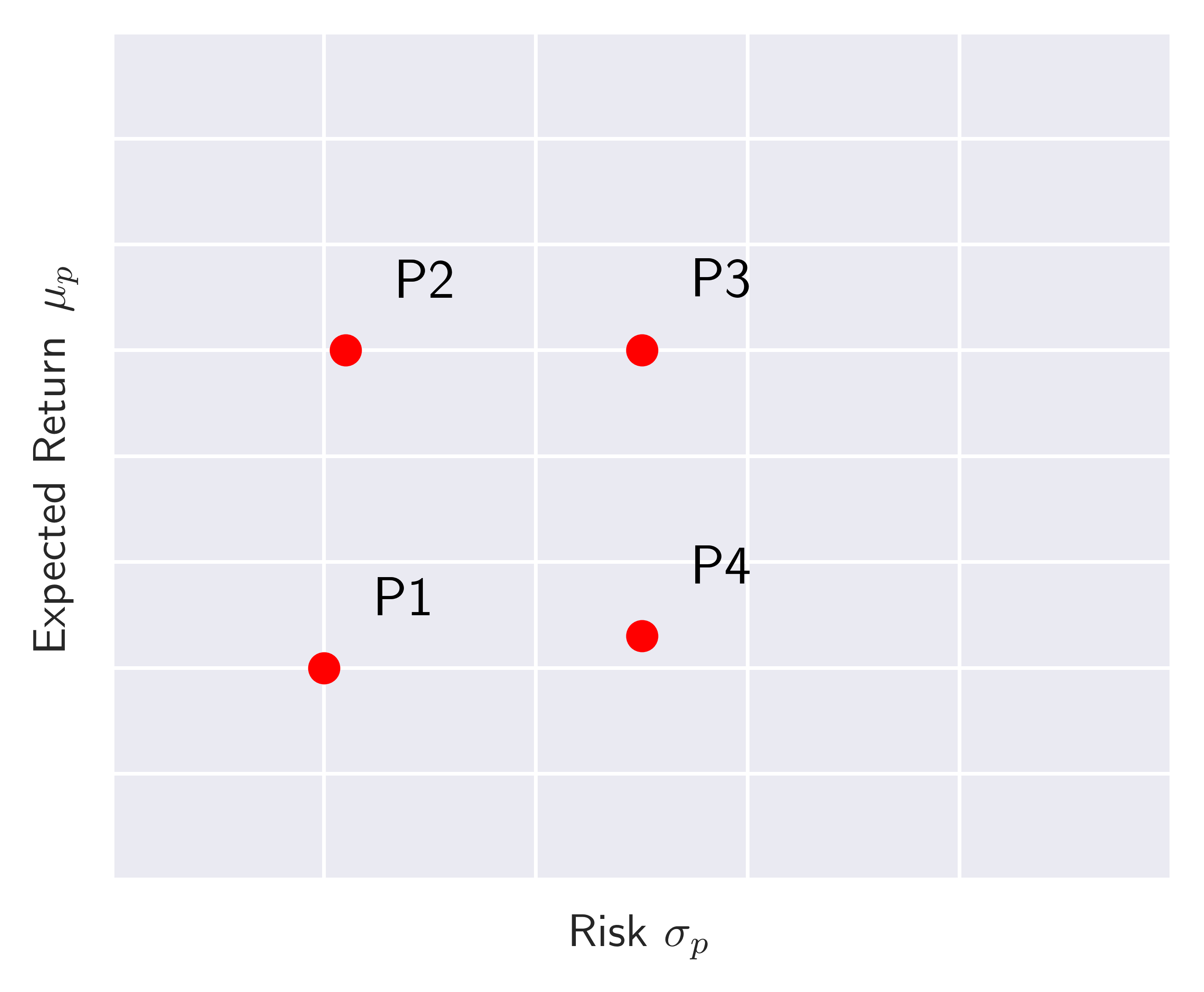 Figure 1. Risk-reward spectrum of four fiducial portfolios.
Assuming that investors tend to care about higher returns with low risk, they would prefer $P3$ over $P4$ or $P2$ over $P1$. Therefore, ideally, every investor would like to move in the North-West direction as this is the direction where one collects more rewards with less risk. In other words, investors care about risk-adjusted returns!
Let’s elaborate more on the risk-reward spectrum by returning to our two asset example (Asset A and B) as it allow us to characterize the portfolio and its properties by a single weight due to the constraint in eq \eqref{w}. In this special case, the expected return of the portfolio and its variance is given by
\[\begin{align} \nonumber \mu_p &= w_A \mu_A + w_B \mu_B,\\\nonumber \\ \label{2ap}\sigma_p^2 &= w_A^2 \sigma_A^2 + w_B^2 \sigma_B^2 + 2 w_A\,w_B\,\sigma_A \sigma_B\, \rho_{AB}, \end{align}\]where $w_B = 1 - w_A$. Now consider that asset A has monthly mean return $\mu_A = 3 \%$ with volatility of $\sigma_A = 6 \%$ while asset B has a mean return of $\mu_B = 1 \%$ with a volatility of $\sigma_B = 3 \%$ and a correlation between the returns of $\rho_{AB} = 0.2$. To get a feeling of how a portfolio made of these assets perform, we can construct the following table
| Portfolio | $w_A$ | $w_B$ | $\mu_p\,\,[\%]$ | $\sigma_p\,\,[\%]$ |
|---|---|---|---|---|
| B-only | 0 | 1 | 1.00 | 3.00 |
| T-S | 0.3 | 0.7 | 1.60 | 3.03 |
| Dutch | 0.5 | 0.5 | 2.00 | 3.61 |
| S-T | 0.7 | 0.3 | 2.40 | 4.47 |
| A-only | 1 | 0 | 3.00 | 6.00 |
| Leveraged A | 1.30 | -0.30 | 3.6 | 7.67 |
Notice that instead of investing on B only, one can potentially obtain more gains by constructing a thirty to seventy (T-S) portfolio without essentially taking more risk. The portfolio theory does not guide us about which portfolio to pick but give us insights on questions such as “How much risk we can handle for a desired level of return?” or “Can we enhance our returns at a given level of risk?”. For example the last row corresponds to a portfolio where asset B has a short position so that the money borrowed from this transaction is used to leverage the long position of asset A. The expected return of this portfolio is higher but so does the volatility (risk) associated with it.
For the two asset case, we can visualize all possible portfolios in the risk-reward spectrum by simply scanning over a grid of $w_A$ (recall $w_B = 1 - w_A$). Notice that in this special case, we are anticipating to characterize a curve in 2-D space (risk-reward) using one affine parameter $w_A$. If we were to work with more than two assets $n > 2$, the space of all possible portfolios would span an area within the risk-reward spectrum.
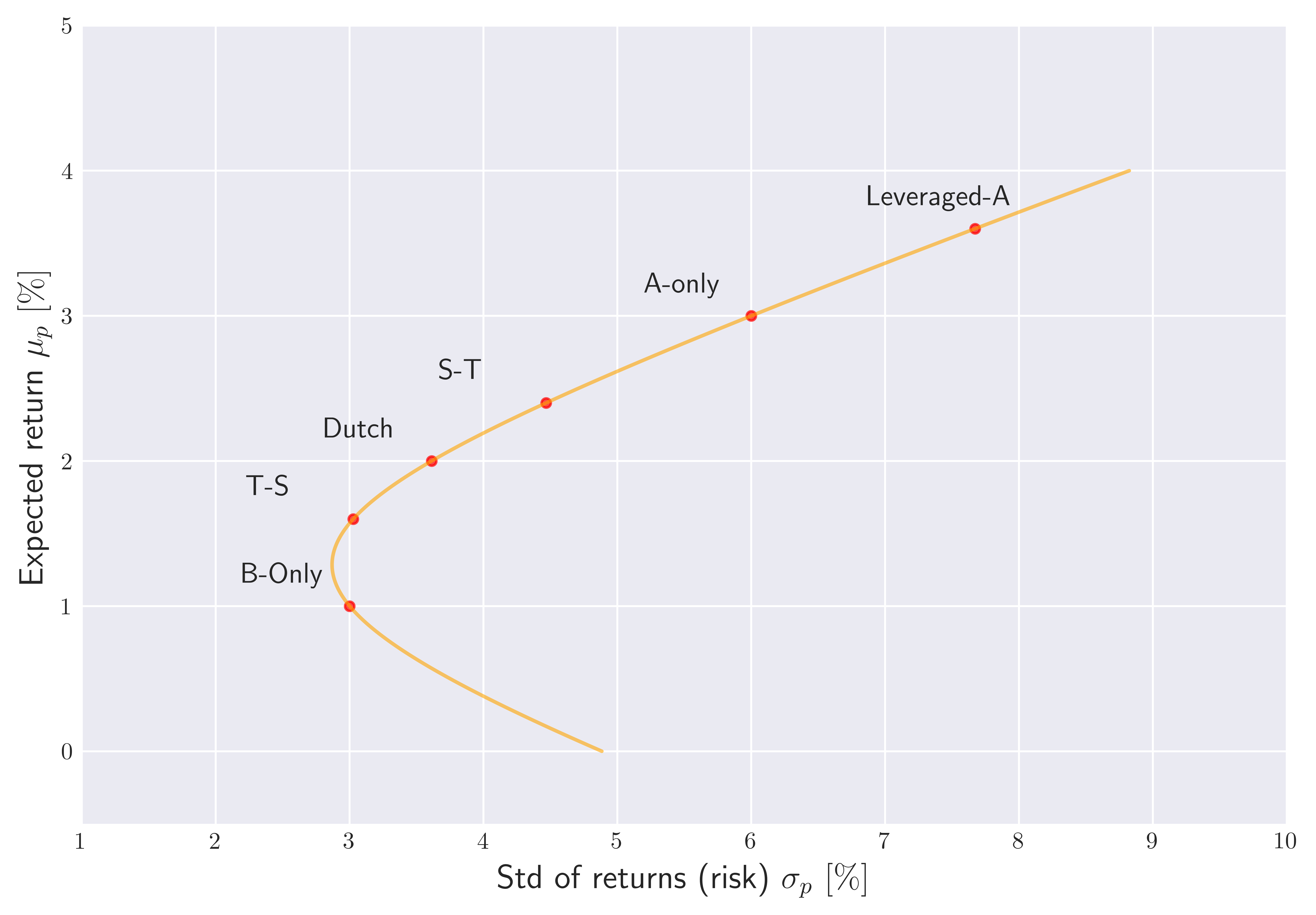 Figure 2. The set of all possible two asset portfolios obtained via scanning through $w_A \in [-0.5,1.5]$: $A$ and $B$. Red dots represent the portfolios we discussed in the table above.
We illustrate these points in Figure 2. We observe the set of all possible portfolios that parametrize the risk-reward trade-off has a parabolic, bullet like shape. This is the famous Markowitz bullet that arise due to non-linear relationship between $\sigma_p$ and $\mu_p$.
Recall that for the two asset case, we can not move away (up/down or left/right) from the orange curve shown in Figure 2. Furthermore, the portfolios that reside on the bottom part of the curve are inefficient as we can move up and left along the curve to work with portfolios that have higher returns and lower risk. The remaining upper part of the Markowitz bullet is therefore corresponds to the efficient frontier that represents the set of portfolios that offer the highest expected return for a given level of risk or conversely the lowest risk for a given expected return. In other words, efficient frontier shows the best possible risk-return trade-offs available from a given set of assets. We will consider more complicated example with $n > 2$ to elaborate more on the significance of the efficient frontier.
Looking at Figure 2., we once again confirm the inefficiency of putting all our money to asset B, as we can potentially adopt the “thirty to seventy” mixture of A and B to leverage our returns while staying almost at the same level of risk. If we are willing to take more risk, we can adopt the “Dutch” portfolio and so on. Notice also that the “Leveraged-A” portfolio appears beyond the “Only -A” portfolio, which makes sense as we leveraged it $w_A = 1.3$ by short selling asset B.
The full Python code to reproduce Figure 2. can be found in Appendix A.
The importance of asset correlations $\rho_{ij}$ : In the two asset example we have been focusing so far, we assumed a fixed correlation between two assets. In the real world, however the correlations between assets are not static and change over time as the market conditions or the factors that affect these conditions change. Therefore, it would be instructive to delve into the two asset example again to gain more insight on the geometry of the risk reward spectrum for a changing $\rho_{ij}$.
For the parameter choices we adapt to generate Figure 2. (e.g $\mu_A = 3$, $\sigma_A = 6$, $\mu_B = 1$, $\sigma_B = 3$), we illustrate the effect of changing correlation on the risk-reward spectrum in Figure 3 for a grid of correlations:
\[\rho_{AB} = [-1,-0.5,0,0.5,1]\]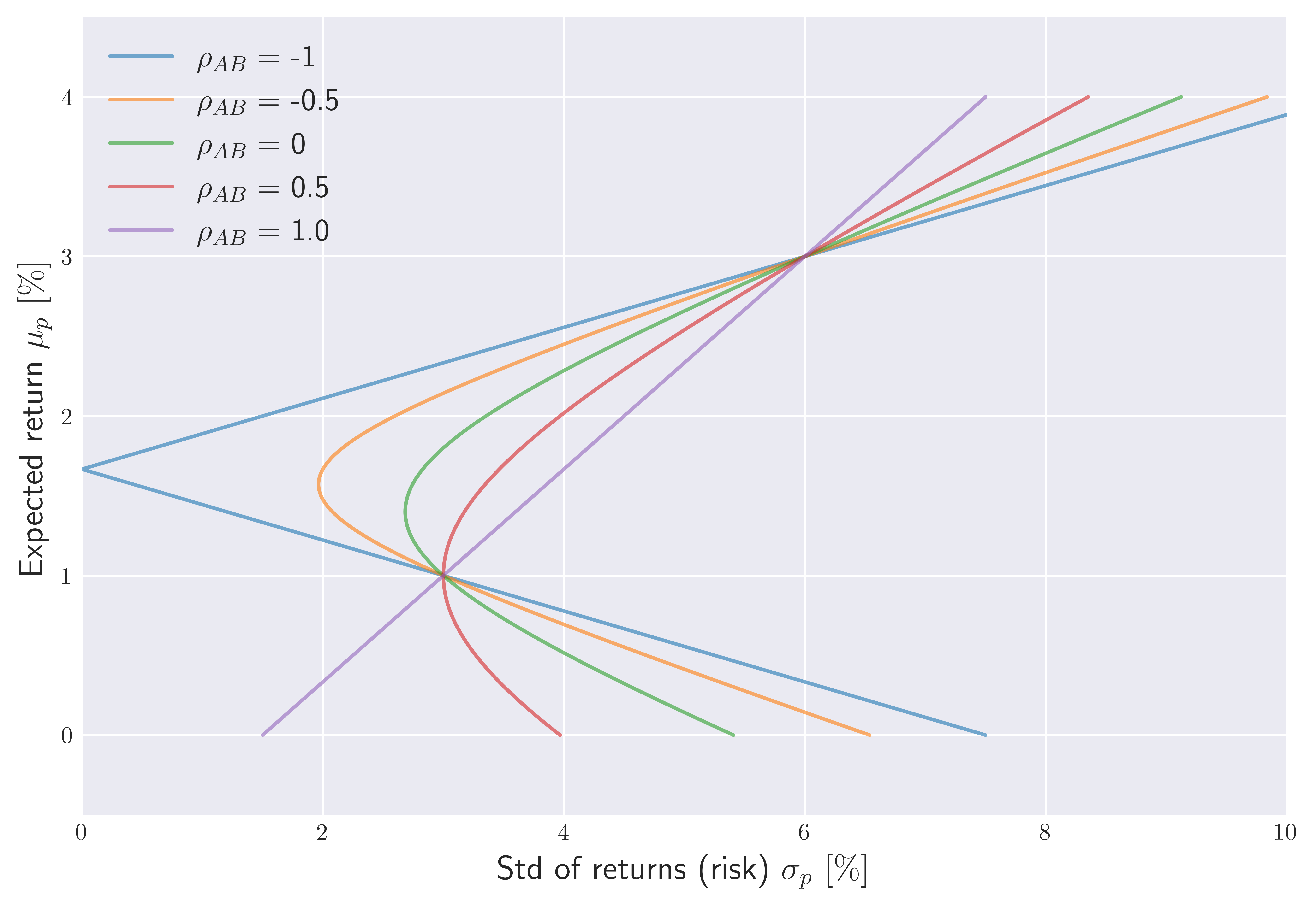 Figure 3. The set of all possible two asset portfolios ($ w_A \in [-0.5,1.5] $) for different choices of correlations between A and B.
We observe that for perfect correlation $\rho_{AB} = 1$, the non-linearity that is present for $0 < \rho_{AB} < 1$ turns into linear relation between risk and reward. Of course in reality, perfect correlation is impossible unless we essentially have the same asset weighted different ways to make up a portfolio. The linear relation we see for this case implies that there is no viable weight combinations that would allow us to reduce risk while gaining more returns from such a portfolio. This behavior can be understood by noting the fact that $w_A$ is always linear in $\mu_p$, see e.g \eqref{2ap} which implies a linear relationship (with a positive slope) between the standard deviation of portfolio and portfolio return $\mu_p$ (or vice versa):
\[\sigma_p = \sqrt{(w_A \sigma_A + w_B \sigma_B)^2} = |w_A (\sigma_A - \sigma_B) + \sigma_B| \propto \frac{\sigma_A - \sigma_B}{\mu_A - \mu_b} \mu_p\]as long as the inequality $w_A > - \sigma_B / (\sigma_A - \sigma_B) = -1$ satisfied. Note that this is the case, as for two asset examples we are considering, we do not allow short positions of A for more than fifth percent of our budget: $w_A \in [-0.5, 1.5]$.
As we reduce the correlation towards the range $0 \leq \rho_{AB} < 1$, the benefits of diversification begin to arise in the risk-reward spectrum, similarly to the situation shown in Figure 2. In this case, the relationship between $\mu_p$ and $\sigma_p$ is non-linear as we advertised before.
On the other hand, when $\rho_{AB}$ becomes negative, the Markowitz bullet gets sharpened further turning into a kinky spear for perfect anti-correlation $\rho_{AB} = -1$. In this case, there are two branches of linear solutions separated by $w_A = \sigma_A / (\sigma_A + \sigma_B) = 1/3$ where $\mu_p = 5/3 \%$ and $\sigma_p = 0$:
\[\begin{align} \sigma_p^{-} &= |w_A (\sigma_A + \sigma_B) - \sigma_B| \propto - \frac{(\sigma_A + \sigma_B)}{\mu_A - \mu_B}\mu_p,\quad\quad w_A < 1/3, \\ \sigma_p^{+} &= |w_A (\sigma_A + \sigma_B) - \sigma_B| \propto + \frac{(\sigma_A + \sigma_B)}{\mu_A - \mu_B}\mu_p,\quad\quad w_A > 1/3. \end{align}\]These facts explain the piece-wise linear risk-reward trade-off that appear in Figure 3 for perfect anti-correlation $\rho_{AB} = -1$. This result is remarkable, as it tells us that there is a way to construct a portfolio where we can get a monthly return of $\mu_p = 5/3 \%$ without any risk. Of course in reality this is not possible as there are no two assets that are perfectly anti-correlated. However, portfolio theory gives us a general idea for maximizing our returns while potentially reducing risk involved with our investments by focusing on less correlated or negative correlated assets.
Mean-Variance Optimization for a large number of assets
For more than two assets $n>2$, mean-variance analysis becomes analytically intractable. In the real world however, portfolio managers generally work with portfolios that contain a large number of assets $n \gg 1$. In this case, all the available set of portfolios do not just lie on a parabolic curve but span an area in the risk-reward spectrum as we advertised earlier.
To illustrate this point, I have analyzed the last two years of (daily) price data (obtained using yfinance library) belonging to the tickers 'ENPH', 'BP', 'PFE', 'NVDA' which exhibit relatively small correlations among each other. Computing approximate monthly mean returns and covariances from the daily frequency data, I have generated 10000 long only portfolios whose weights $w_i \in [0,1]$ are drawn from a uniform distribution. The risk reward spectrum of the resulting portfolios constructed from these assets are shown in Figure 4. where the color coding for each point is determined using a commonly used performance metric called Sharpe ratio with bright regions corresponding to a relatively large sharpe ratio:
where $r_f$ is the risk-free interest rate, namely the interest rate achievable without any risk (e.g. via Treasury Bills in the USA). As implied by the eq. \eqref{sr}, Sharpe ratio is commonly reported metric for portfolio performance that essentially measures return per unit risk.
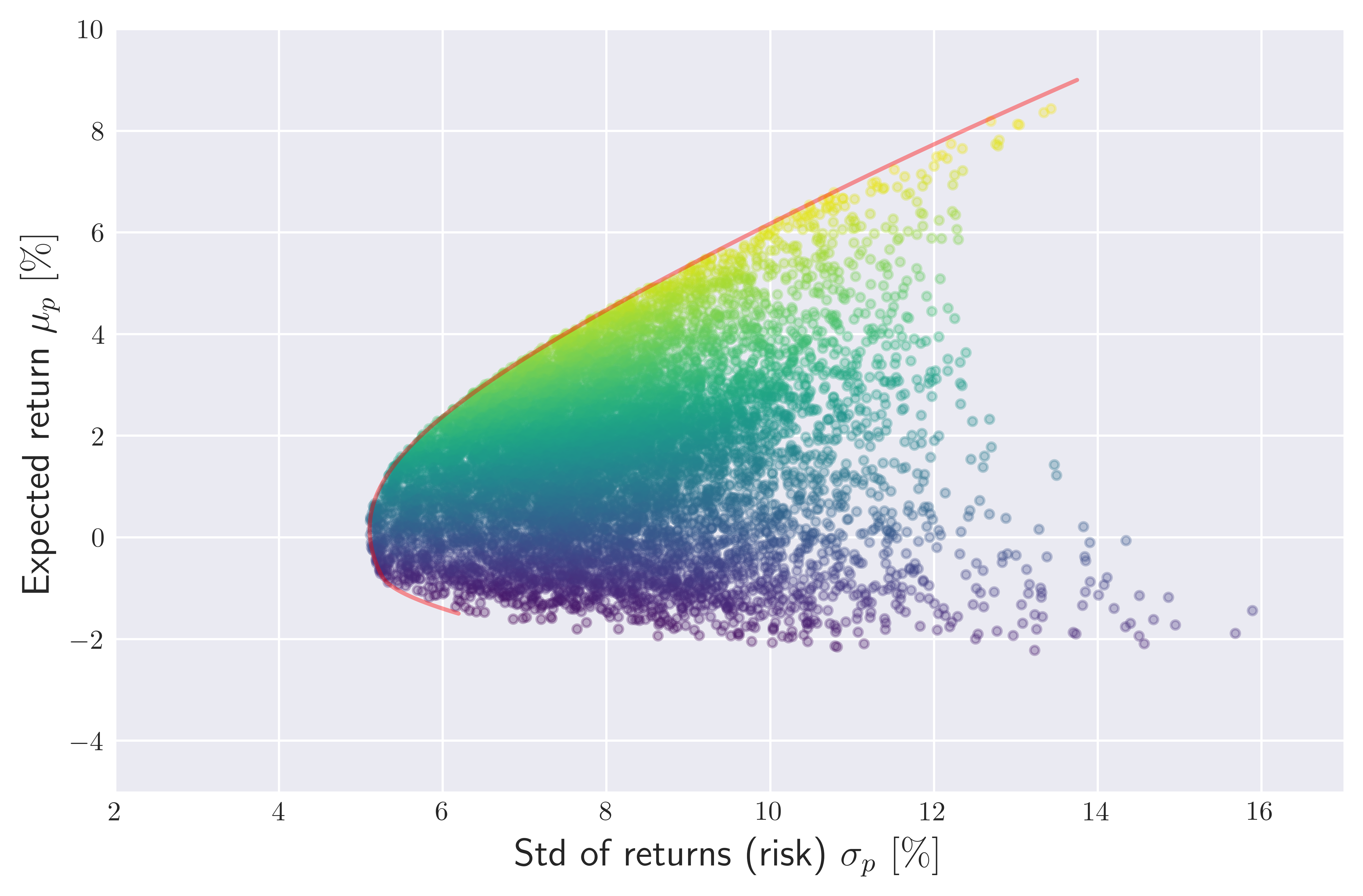 Figure 4. The risk-reward spectrum (monthly) of all possible long-only portfolios ($w_i \in [0,1] $) containing
 'ENPH', 'BP', 'PFE', 'NVDA'. The color of each point is represented with its Sharpe ratio \eqref{sr} with bright points corresponding the larger value of the latter. We have assumed risk free rate to be vanishing, $r_f = 0$.
Now consider that we have a portfolio that resides deep inside the Markowitz bullet and ask ourselves if this is an efficient portfolio. In particular how can we achieve the same return with less risk? The answer to this question obviously depends on the portfolio weights which can be framed as an optimization problem of finding the weights $\vec{w}$ that minimize the portfolio risk $\sigma_p$ for a desired level $R_d$ of portfolio return, assuming that we have the estimates for the expected returns $\vec{\mu}$ and covariances ${\bf \Sigma}$ of the assets:
\[\begin{align} \nonumber \min_{\vec{w}}\,\,\quad & \vec{w}^{T}\cdot ({\bf \Sigma}\cdot \vec{w}), \\\nonumber \\\nonumber \textrm{subject to}\,\,\,\quad & \vec{w}^{T} \cdot \vec{\mu} = R_d \\\nonumber \\ \textrm{and} &\,\,\quad \sum_{i = 1}^{n} w_i = 1. \end{align}\]This is a quadratic optimization problem that can be solved for example by means of Lagrange multiplier methods or critical line algorithm originally proposed by Markowitz himself. Nowadays, we have many tools to tackle such problems. For example, we can utilize Python’s built-in .minimize() method from scipy.optimize library for this purpose.
For the shown range $\mu_p$ values in Figure 4., this optimization problem provides us the efficient frontier (shown by the top part of the red curve), representing portfolios that exhibit the smallest available risk for a given expected return $\mu_p$.
In Appendix B, I provide the full Python code that can be used to reproduce Figure 4, including the efficient frontier using the quadratic optimization problem above.
Conclusions
Markowitz’s portfolio theory provides a grounding mathematical framework for the concept of risk reduction by diversification. When constructing a portfolio, investors should seek for assets that have less correlation in order to mitigate the risk involved with their investments. In other words, it tells us that rather than caring only about returns, investors should analyze their portfolios risk-return trade-off for making better informed investment decisions.
References
- Finance Theory 1 Lectures, by Prof. Andrew Lo, MIT, Sloan School of Management, 2008.
Appendix A: Code to reproduce Figure 2.
1
2
3
4
5
6
7
8
9
10
11
12
13
14
15
16
17
18
19
20
21
22
23
24
25
26
27
28
29
30
31
32
33
34
35
36
37
38
39
40
41
42
43
44
45
46
47
48
49
50
51
52
53
54
55
56
57
58
59
60
61
62
63
64
65
66
67
68
69
70
71
72
73
74
75
76
77
import numpy as np
import matplotlib as mpl

import matplotlib.pyplot as plt

mpl.rcParams['text.usetex'] = True

#For inline plotting
%matplotlib inline
%config InlineBackend.figure_format = 'svg'

plt.style.use("seaborn-v0_8-dark")

#######

def get_portolfio_performance(mu,sigma,rho,w):

    '''Helper function to output expected return and std of a two asset portfolio given
       an array of expected individual asset returns (mu),
       volatility (sigma), weights (w) and off-diagonal correlation (rho)
    '''

    mu_p = w.dot(mu)

    sigma_p = np.sqrt((w**2).dot(sigma**2) + 2 * w.prod() * sigma.prod() * rho)

    return mu_p, sigma_p

# array of asset returns and volatility
mu = np.array([3,1])
sigma = np.array([6,3])

# assumed correlation between assets
rho = 0.2

# Example portfolios
w_dict = {'B-Only': np.array([0,1]), 'T-S': np.array([0.3,0.7]), 'Dutch': np.array([0.5,0.5]),
          'S-T': np.array([0.7,0.3]), 'A-only': np.array([1,0]), 'Leveraged-A': np.array([1.3,-0.3])}

# Generate a grid of w_A values that we will iterate over
wa_min = -0.5
wa_max = 1.5
wa_space = np.linspace(wa_min, wa_max, 1000)

# empty array of risk-reward pairs
risk_vs_reward = np.full(shape = (1000,2), fill_value=0.)

# compute portfolio return and risk for each w_A and corresponding w_B
for idx, wa in enumerate(wa_space):

    wb = 1 - wa

    w = np.array([wa,wb])

    mu_p, sigma_p = get_portolfio_performance(mu,sigma,rho,w)

    risk_vs_reward[idx,0] = sigma_p
    risk_vs_reward[idx,1] = mu_p


fig, axes = plt.subplots(figsize = (9,6))

axes.plot(risk_vs_reward[:,0], risk_vs_reward[:,1], c = 'orange', alpha =0.6)

for portfolio, weights in w_dict.items():

    mu_p, sigma_p = get_portolfio_performance(mu,sigma,rho,weights)
    axes.scatter(sigma_p, mu_p, marker = 'o', s = 15, c = 'red', alpha = 0.7)
    axes.annotate(portfolio, xy = (sigma_p-0.8,mu_p+0.16), size = 12)


axes.set_xlabel(r'Std of returns (risk) $\sigma_p\,\, [\%]$', fontsize = 14)
axes.set_ylabel(r'Expected return $\mu_p\,\, [\%]$', fontsize = 14)

axes.set_xlim(1,10)
axes.set_ylim(-0.5,5)
axes.grid()
Appendix B: Code to reproduce Figure 4.
1
2
3
4
5
6
7
8
9
10
11
12
13
14
15
16
17
18
19
20
21
22
23
24
25
26
27
28
29
30
31
32
33
34
35
36
37
import numpy as np
import matplotlib as mpl
import matplotlib.pyplot as plt
import yfinance as yf
import datetime as dt
from scipy.optimize import minimize

mpl.rcParams['text.usetex'] = True

#For inline plotting
%matplotlib inline
%config InlineBackend.figure_format = 'svg'

plt.style.use("seaborn-v0_8-dark")

def get_hist_data(stocks, start, end):
    '''Helper function that gets the stock data from yfinance
       to return returns, mean_returns and covariance Matrix of returns'''
    tickers_df = yf.download(stocks, start = start, end = end)

    close_df = tickers_df['Close']

    returns_df = close_df.pct_change().dropna()

    mean_returns_df = returns_df.mean()
    cov_Matrix_df = returns_df.cov()

    return returns_df, mean_returns_df, cov_Matrix_df

def portfolio_performance(mu,covM,w):
    '''Helper function to obtain portfolio performance (n assets)
       input: array of returns, covariance matrix and weights'''

    mu_p = w.dot(mu)
    sigma_p =np.sqrt(w.dot(covM).dot(w))

    return mu_p, sigma_p
1
2
3
4
5
6
7
8
9
10
11
12
13
14
15
16
17
18
19
20
21
22
23
24
25
26
27
28
29
30
31
32
33
34
35
36
37
38
39
40
41
42
43
44
45
46
47
48
# get returns, daily mean returns and covariances

tickers = ['ENPH', 'BP', 'PFE', 'NVDA']

end_date = dt.datetime.now()
start_date = end_date - dt.timedelta(days = 736)

returns, mean_returns_df, covM_df = get_hist_data(tickers, start = start_date, end = end_date)

# monthly returns by multiplying mean daily returns
# with the number of trading days in a month
mon_ret =(mean_returns_df * 21).to_numpy()
mon_cov = (covM_df * 21).to_numpy()

# number of portfolio sims
N_sim = 10000

# number of assets
D = len(mon_ret)

# initialize portfolio variables for all sims
port_returns = np.zeros(N_sim)
port_risks = np.zeros(N_sim)
sharpe = np.zeros(N_sim)

for i in range(N_sim):

    rand_w = np.random.random(D) # random weights between [0,1] drawn from uniform dist.

    # sum of weigths to be used to normalize
    total_w = np.sum(rand_w)

    # get the normalized weigths that sum up to 1 and shuffle
    normalized_w = np.array([num/total_w for num in rand_w])
    np.random.shuffle(normalized_w)

    # get portfolio perfomence
    mu_p, sigma_p = portfolio_performance(mon_ret, mon_cov, normalized_w)

    # assign risk and return of the portfolio for each simulation
    port_returns[i] = mu_p
    port_risks[i] = sigma_p

    # get the sharpe ratio of each portfolio sim
    sharpe[i] = mu_p / sigma_p

# scale sharpe ratio so that minimum is 0 and maximum is 1
minmax_scaled_sharpe = (sharpe - sharpe.min())/(sharpe.max()- sharpe.min())
1
2
3
4
5
6
7
8
9
10
11
12
13
14
15
16
17
18
19
20
21
22
23
24
25
26
27
28
29
30
31
32
33
34
# efficient frontier for a given target return through optimization
def efficient_frontier(R_p):

    def objective(w):

        return np.sqrt(w.dot(mon_cov).dot(w))

    min_result = minimize(fun = objective, x0 = np.ones(D)/D,  bounds = [(0.0,1.)]*4, method = 'SLSQP', constraints = [{'type': 'eq', 'fun': lambda w: 1 - w.sum()},
                                                                                                              {'type': 'eq', 'fun': lambda w: w.dot(mon_ret) - R_p}])
    # .x returns weights .fun would return risk
    return min_result.x

efficient_returns = np.zeros(250)
efficient_risks = np.zeros(250)

for idx, target in enumerate(np.linspace(-0.015,0.09,250)):

    w = efficient_frontier(target)

    efficient_returns[idx], efficient_risks[idx] = portfolio_performance(mon_ret, mon_cov, w)

fig, axes = plt.subplots(figsize = (8,5))

axes.scatter(port_risks * 100, port_returns * 100, alpha = 0.3, c = minmax_scaled_sharpe, s = 10,  cmap = 'viridis')

axes.plot(efficient_risks * 100, efficient_returns * 100, alpha = 0.4, c = 'red')

axes.set_xlabel(r'Std of returns (risk) $\sigma_p\,\, [\%]$', fontsize = 14)
axes.set_ylabel(r'Expected return $\mu_p\,\, [\%]$', fontsize = 14)

axes.set_xlim(2, 17)
axes.set_ylim(-5,10)

axes.grid()