Option pricing in a jumpy world
I discuss risk-neutral pricing of option contracts when the underlying stock follows a jump-diffusion process.
Previously, I discussed the dynamics of stocks and derived the differential equation for its options when the underlying follows a jump-diffusion process. In this post, I would like to extend the discussion towards a practical direction of finding a pricing formula for the option with an aim to assess phenomenology of jump diffusion models.
Recall that under the risk-neutral measure, in a jumpy market the stock dynamics obeys the following SDE:
\[\begin{equation}\label{jdp} \frac{\mathrm{d}S_t}{S_t} = (r - \lambda \mathbb{E}\left[\mathrm{e}^J-1\right])\mathrm{d}t + \sigma\,\mathrm{d}W^{\mathbb{Q}}_t + (\mathrm{e}^J - 1)\, \mathrm{d}N_t, \end{equation}\]where $\mathrm{d}N_t$ is the incremental Poisson process that counts the number of occurrence of jumps between times $t$ and $t + \mathrm{d}t$ and $J$ is an random variable (independent of the Poisson and Wiener process) representing the size of the discontinuous jumps. A jump occurs $\mathrm{d}N_t = 1$ with a real-world probability $\lambda\, \mathrm{d}t$ otherwise $\mathrm{d} N_t = 0$ with probability $1 - \lambda\,\mathrm{d}t$. Here, the jump process is assumed to be independent of the diffusive part $\mathrm{d}W^{\mathbb{Q}}$.
We can price a contingent claim (such as a call/put option) by taking the discounted expectation of its pay-off (at the maturity) under the risk-neutral/martingale measure:
\[\begin{equation}\label{rop} \frac{C_t(S_t)}{Z_t} = \mathbb{E}_{\mathbb{Q}}\left[\frac{C_T(S_T)}{Z_T} \bigg |\, \mathcal{F}_t\right], \end{equation}\]where $Z_t = e^{-r(T-t)}$ is a money market account/riskless bond that is assumed to be deterministic. To evaluate the expression \eqref{rop}, we need to determine the terminal distribution of the stock price by integrating \eqref{jdp}. For this purpose, we first aim to understand what happens to the log process when a jump occurs $\mathrm{d}N_t = 1$. The process \eqref{jdp} tells us that the log-return at time $t + \Delta t$ for an investment on the stock at time $t$ is just given by the jump parameter $J$:
\[\begin{equation} \frac{\Delta S_t}{S_t} = \frac{S_{t + \Delta t} - S_t}{S_t} = \mathrm{e}^J - 1, \quad\quad \Longrightarrow \quad\quad \Delta (\ln S_t) = \ln \left(\frac{S_{t + \Delta t}}{S_t}\right) = J. \end{equation}\]On the other hand, we know that in the absence of jump $\mathrm{d}N_t = 0$, stock follows a standard geometric Brownian motion (GBM) such that applying Ito’s lemma to the log-process, the latter acquires a drift adjustment of the form $(-\sigma^2 / 2) \mathrm{d}t$. Therefore, in the presence of jumps the log process $\ln S_t$ satisfies the following SDE:
\[\begin{equation}\label{ljdp} {\mathrm{d}\ln S_t} = \left(\mu_\mathbb{Q} - \frac{\sigma^2}{2}\right)\mathrm{d}t + \sigma\,\mathrm{d}W^{\mathbb{Q}}_t + J\, \mathrm{d}N_t, \end{equation}\]where we defined the risk-neutral drift of the GBM
\[\mu_\mathbb{Q} = r - \lambda \mathbb{E}\left[\mathrm{e}^J-1\right].\]Note that we could reach at the same result in \eqref{ljdp} by utilizing modified Ito’s lemma that takes into account the jumps.
An important that the expression \eqref{ljdp} tells us is that, if we consider the process for log-returns, there is no interaction between the Brownian part and the jumpy part. In other words, \eqref{ljdp} reflects that if no jump occurs log-returns will just evolve as in the continuous case and if a jump occurs in the stock price $S_{t + \Delta t} = S_t \mathrm{e}^J$, this is equivalent to adding a $J$ to log-returns or: $\ln S_{t + \Delta t} = \ln S_t + J $. Integrating the whole process until the maturity $T$ of the option contract, the terminal distribution of the log-stock price is thus given by
\[\begin{equation}\label{tdls} \ln S_T \sim \ln S_0 + \left(\mu_\mathbb{Q} - \frac{\sigma^2}{2}\right)\, T + \sigma\, \sqrt{T}\, Z_W + \sum_{j = 1}^{N(T)} J_i. \end{equation}\]where $Z_W \sim N(0,1)$ is a standard normal variable, and $J_j$ are independent variables distributed according to a jump distribution, and $N(T)$ is the number of jumps, which is itself a random variable. Using \eqref{tdls}, we can in principle price a contract with a known terminal value in terms of the value of its underlying $O = O(S_T)$ by using Monte Carlo techniques. All we need to do is just draw the number of jumps, the size of each of the jumps from a distribution and similarly the Brownian part to get the final spot, and evaluate the option. We illustrate the stock dynamics that follows a jump diffusion process under the Merton’s classical model (see below) in Figure 1 (see Appendix A).
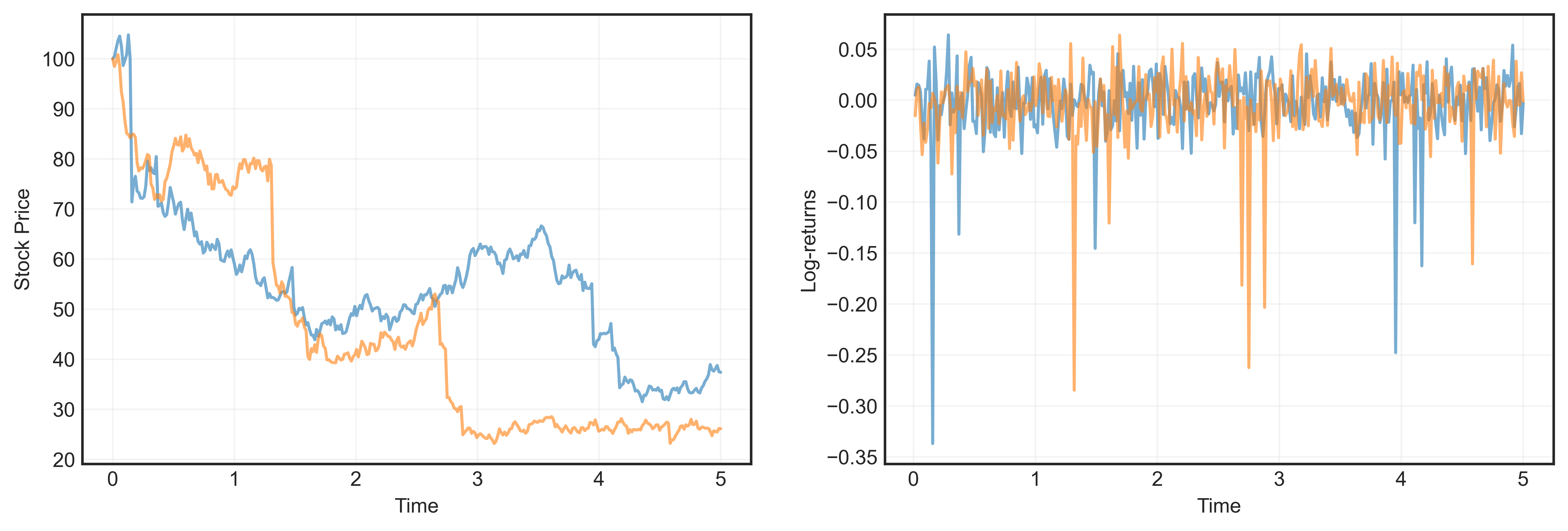 Figure 1. Monte Carlo simulation of the stock price (left) and the corresponding log-returns (right) for two (unlucky!) simulation paths within the Merton’s Model. We take $S_0 = 100$, $r = 0.05$, $\sigma = 0.2$, $\lambda = 1$, $\mu_J = -0.2$, $\sigma_J = 0.1$. The location of the jumps are clearly visible from the time evolution of log-returns (right).
In order to proceed analytically, we need to make some assumptions about the nature of jumps. One possibility is that each jump have identical size $J$ so that the last term in \eqref{tdls} read as $N(T) J$. Of course, a single jump amplitude is not realistic and in fact we can do better. For example, two popular choices that assume a continuous jump distribution are:
- Classical Merton’s model [Merton 1976]: The jump amplitude is normally distributed with mean $\mu_J$ and standard deviation $\sigma_J$:
- Kou’s non-symmetric double exponential model [Kou 2002, Kou and Wand 2004] :
where $p_1, p_2$ are positive real numbers that satisfy $p_1 + p_2 = 1$. To be able to integrate $x$ over the real line it is required to have $\alpha_1 > 1$ and $\alpha_2 > 0$. The parameters $\alpha_1$ and $\alpha_2$ represent the different decay rates for the right and left tails of the distribution. Note that the distribution itself is continuous at $x = 0$ (no jump) but not differentiable there. For some details on this parametrization of non-symmetric double exponential distribution and its Python implementation see Appendix B.
To illustrate the perks of the jump diffusion models, here I will focus on the Merton’s model and study the non-symmetric double exponential model elsewhere. For this purpose we draw each $J_i$ from a normal distribution $N(\mu_J, \sigma_J^2)$ such that $J_i = \mu_J + \sigma_J Z_j$ where $Z_j$’s are iid standard normal. The terminal distribution of the log stock process is then
\[\begin{equation}\label{mm} \ln S_T \sim \ln S_0 + \left(\mu_\mathbb{Q} - \frac{\sigma^2}{2}\right)\, T + \sigma\, \sqrt{T}\, Z_W + \sum_{j = 1}^{N(T)} (\mu_j + \sigma_J Z_j). \end{equation}\]Since $Z_j$’s are independent of each other, as well as from the random variable associated with the diffusive part $Z_W$, the sum
\(\begin{equation} \sigma \sqrt{T} Z_W + \sum_{j = 1}^{N(T)} \sigma_J Z_j, \end{equation}\) can be combined into another normal variable with a variance equivalent to
\[\begin{equation} \mathbb{V}\left[\sigma \sqrt{T} Z_W + \sum_{j = 1}^{N(T)} \sigma_J Z_j\right] = \sigma^2 T\, \mathbb{V}[Z_W] + \sum_{j = 1}^{N(T)} \sigma_J^2\, \mathbb{V}[Z_j] = \left(\sigma^2 + N(T) \frac{\sigma_J^2}{T}\right) T \equiv \bar{\sigma}^2\, T. \end{equation}\]This allows us re-write the terminal distribution \eqref{mm} in a convenient way as:
\[\begin{equation}\label{mmf} \ln S_T \sim \ln S_0 + \left(\mu_\mathbb{Q} - r\right)\, T + N(T)\left(\mu_J + \frac{\sigma_J^2}{2}\right) + \left(r - \frac{\bar{\sigma}^2}{2}\right)\, T + \bar{\sigma}\, \sqrt{T}\, \bar{Z} . \end{equation}\]Notice that for a given $N(T)$, this is the terminal distribution of a stock in the Black-Scholes world with a modified volatility $\bar{\sigma}$ and initial stock price
\[\bar{S}_0 = S_0\, \mathrm{e}^{(\mu_\mathbb{Q} - r) T + N(T) (\mu_J + \sigma_J^2 /2)}.\]Note however, $N(T)$ is itself a random variable that takes integer values. We may therefore expect the price of the option to be an infinite sum over these possible number of jump values, weighted appropriately by the laws of Poisson process. To see this, we first note the price of the option contract at $t = 0$ using \eqref{rop} as
\[\begin{equation}\label{ropf} \frac{C_0}{\mathrm{e}^{-r T}} = \mathbb{E}_{\mathbb{Q}}\left[ \textrm{max}(S_T - K, 0) \right], \end{equation}\]where we used the fact that conditioning on $\mathcal{F}_0$ is equivalent to conditioning on no information as the process has not revealed itself at the inception of the contract. The expectation in \eqref{ropf} is over the joint distribution of the diffusive $\bar{Z}$ and the Poisson process (which is in fact over a real world probability measure $\mathbb{P}$) that are independent. Conditioned on the latter, we therefore have
\[\begin{align} \nonumber {C_0} &= \mathrm{e}^{-r T}\sum_{n = 0}^{\infty}\,\mathbb{E}_{\mathbb{Q}}\left[ \textrm{max}(S_T - K, 0) | N(T) = n \right]\,\mathbb{P}(N(T) = n),\\ &= \sum_{n = 0}^{\infty} \frac{(\lambda T)^{n}}{n!}\, \mathrm{e}^{-\lambda T} C_{BS} (\bar{S}_0(n), r, \bar{\sigma}(n), T, K),\label{ropff} \end{align}\]where $C_{BS}$ is the Black-Scholes price of the option with initial spot and volatility
\[\begin{align} \nonumber \bar{\sigma}(n) &= \sqrt{\sigma^2 + \frac{n \sigma_J^2}{T}},\\ \nonumber \bar{S}_0(n) &= S_0\, \mathrm{e}^{-\lambda (m - 1) T + n \ln m},\\ m \equiv&\, \mathbb{E}\left[\mathrm{e}^{J}\right] = \mathrm{e}^{\mu_J + \sigma_J^2 / 2}. \end{align}\]A final simplification to \eqref{ropff} arise by noticing the following property of Black-Scholes price:
\[\begin{align} \nonumber C_{BS}(S_0(n),r,\bar{\sigma}(n),T,K) &= \mathrm{e}^{-\lambda (m - 1) T + n \ln m}\, C_{BS}(S_0,\bar{r}(n),\bar{\sigma}(n),T,K),\\ \bar{r}(n) &\equiv r - \lambda (m - 1) + \frac{n \ln m}{T}. \end{align}\]where we made use of the standard definition
\[\begin{align} \nonumber d_2(\bar{S}_0,r,\bar{\sigma}) &= \frac{\ln(\bar{S}_0/K) + \left(r - \bar{\sigma}^2 / 2\right) T}{\bar{\sigma}\sqrt{T}},\\ \nonumber &= \frac{\ln({S}_0/K) + \left((r - \lambda (m - 1)+ n \ln m / T) - \bar{\sigma}^2 / 2\right) T}{\bar{\sigma}\sqrt{T}},\\ \nonumber &= \frac{\ln({S}_0/K) + \left(\bar{r} - \bar{\sigma}^2 / 2\right) T}{\bar{\sigma}\sqrt{T}},\\ &= d_2(S_0, \bar{r}, \bar{\sigma}), \end{align}\]together with
\[\begin{align} C_{BS}(S,r,\sigma,T,K) = S\, N(d_2 + \sigma \sqrt{T}) - K\, \mathrm{e}^{-r T}\, N(d_2). \end{align}\]Compiling this information in \eqref{ropff}, we obtain the option price as an infinite sum of Black-Scholes option prices weighted by the probability of $n$ jumps over the life-time $T$ of the contract with initial stock price $S_0$ and $\bar{\sigma}(n)$, $\bar{r}(n)$ can be interpreted as the volatility and growth rate of the stock per unit time if $n$ jumps have taken place:
\[\begin{align} {C_0} &= \sum_{n = 0}^{\infty} \frac{(\lambda' T)^{n}}{n!}\, \mathrm{e}^{-\lambda' T} C_{BS} ({S}_0, \bar{r}(n), \bar{\sigma}(n), T, K),\label{ropfff} \end{align}\]where
\[\begin{align} \nonumber \bar{\sigma}(n) & =\sqrt{\sigma^2+n \sigma_J^2 / T}, \\ \nonumber \bar{r}(n) & =r-\lambda(m-1)+n \log m / T, \\ \lambda^{\prime} & =\lambda m. \end{align}\]This is it, we derived a formula for arbitrage-free price of call options (and of course puts via put-call parity) on a non-dividend-paying stock in a jumpy world. Although we did not show that \eqref{ropfff} is the only arbitrage-free price, we know that it is arbitrage-free. This arbitrage-free price was arrived at by taking an equivalent martingale (risk-neutral) measure obtained by changing the drift of the diffusive part of the stock evolution. The important point of the analysis above is that we change the measure on our space of stock paths by letting $\lambda$ be whatever we want as long as it is non-zero. We thus have an infinite number of pricing measures: first we choose a value for $\lambda$, and then we enact a drift change on the Brownian motion to make the adjusted measure a martingale. As the implied prices have been arrived at by risk-neutral expectation from an equivalent martingale measure, they are arbitrage-free. We thus have an uncountable infinity of arbitrage-free prices.
References
1. “The concepts and practice of mathematical finance”, Second Edition, Mark S. Joshi.
2. “Mathematical Modeling and Computation in Finance”, World Scientific, Cornelis W. Oosterlee and Lech A. Grzelak.
Appendix A: Jump-diffusive stock paths via Monte Carlo simulation
We implement a helper function that generates stock paths for a jump diffusion process using monte-carlo methods below. The function returns the price paths as well as the associated log-returns and optionally plots them.
1
2
3
4
5
6
7
8
9
10
11
12
13
14
15
16
17
18
19
20
21
22
23
24
25
26
27
28
29
30
31
32
33
34
35
36
37
38
39
40
41
42
43
44
45
46
47
48
49
50
51
52
53
54
55
56
57
58
59
60
61
62
63
64
65
66
67
68
69
70
71
72
73
74
import numpy as np
import matplotlib.pyplot as plt

#For inline plotting
%matplotlib inline
%config InlineBackend.figure_format = 'svg'

# set plot properties to seaborn globally
plt.style.use("seaborn-v0_8-white")

def monte_carlo_jump_diffusion(S0, mu, sigma, lambd, mu_J, sigma_J, T, num_ts, num_sim, plot=False):
    """
    Simulates Monte Carlo paths for a stock price process under the Merton jump-diffusion model,
    using a fully vectorized approach for efficiency.

    Parameters:
        S0      : float  - Initial stock price
        mu      : float  - Drift rate (risk-free)
        sigma   : float  - Volatility
        lambd   : float  - Poisson jump intensity (average number of jumps per year)
        mu_J    : float  - Mean of jump size (log-normal mean)
        sigma_J : float  - Std dev of jump size (log-normal std)
        T       : float  - Total time horizon (years)
        num_ts  : int    - Number of time steps
        num_sim : int    - Number of Monte Carlo simulations
        plot    : bool   - If True, plots a subset of the generated stock price paths

    Returns:
        S_paths : ndarray - Simulated stock price paths of shape (M, N+1)
        log_returns : ndarray - Simulated log-returns paths of shape (M, N)
    """

    dt = T / float(num_ts)  # Time step size

    times = np.linspace(0, T, num_ts)  # Time grid

    # Generate standard Brownian motion increments
    W_t = np.random.randn(num_sim, num_ts - 1)

    # Generate Poisson process increments
    N_t = np.random.poisson(lambd * dt, size = (num_sim, num_ts - 1))

    # Generate jump sizes (normal distributed jumps)
    J_t = np.random.normal(mu_J, sigma_J, size = (num_sim, num_ts - 1))

    # Expected jump factor: E[e^J]
    expected_jf = np.exp(mu_J + 0.5 * sigma_J**2)

    # Compute log returns as a vectorized operation
    log_returns = (mu - lambd * (expected_jf-1) -  (0.5 * sigma**2)) * dt + (sigma * np.sqrt(dt) * W_t) + N_t * J_t

    # Compute cumulative sum of log returns along time axis
    log_price_paths = np.cumsum(log_returns, axis=1)

    # Convert log returns to stock prices
    S_paths = S0 * np.exp(np.hstack([np.zeros((num_sim, 1)), log_price_paths]))  # Insert S0 at t=0

    # Plot if requested
    if plot:

        _, axes = plt.subplots(1,2, figsize=(13, 4))
        axes[0].plot(times, S_paths.T, alpha = 0.6)  # Plot 10 sample paths
        axes[0].set_xlabel('Time')
        axes[0].set_ylabel('Stock Price')
        axes[0].grid(alpha = 0.2)

        axes[1].plot(times[1:], log_returns.T, alpha = 0.6)  # Plot 10 sample paths
        axes[1].set_xlabel('Time')
        axes[1].set_ylabel('Log-returns')
        axes[1].grid(alpha = 0.2)
        plt.savefig('mc_jdp.png', bbox_inches= 'tight', format= 'png', dpi=720)

    return times, S_paths, log_returns
Calling the function with the parameters below, we simulate two paths as in Figure 1.
1
2
3
4
5
6
7
8
9
10
11
S0 = 100       # Initial stock price
mu = 0.05      # diffusion drift (r: risk-free rate)
sigma = 0.2    # diffusion volatility
lambd = 1.    # Jump intensity
mu_J = -0.2   # Mean jump size
sigma_J = 0.1  # Std dev of jump size
T = 5          # Time horizon
num_ts = 350        # Number of time steps (daily)
num_sim = 2      # Number of Monte Carlo simulations

time_grid, S_paths, log_returns = monte_carlo_jump_diffusion(S0, mu, sigma, lambd, mu_J, sigma_J, T, num_ts, num_sim, plot=True)
Appendix B: Non-symmetric double exponential distribution
Given that the decay rates $\alpha_1$ and $\alpha_2$ are positive definite, we first note that $p_1 + p_2 = 1$ is required to be able to interpret the pdf in \eqref{nsde} as a density:
\[\begin{equation} \int_{-\infty}^{\infty}\, f_J(x)\, \mathrm{d}x = 1, \quad \rightarrow \quad p_1\, \alpha_1\, (-\frac{\mathrm{e}^{-\alpha_1\,x}}{\alpha_1}\Bigg|^{\infty}_0 + p_2\, \alpha_2\, (\,\frac{\mathrm{e}^{\alpha_2\,x}}{\alpha_2}\Bigg|^{0}_{-\infty} = 1, \quad \Rightarrow \quad p_1 + p_2 = 1. \end{equation}\]We can also compute the expected jump factor $\mathrm{e}^J$ using:
\[\begin{equation} \mathbb{E}\left[\mathrm{e}^J\right] = \int_{-\infty}^{\infty}\, e^{x} f_J(x)\, \mathrm{d}x, \quad \rightarrow \quad \mathbb{E}[\mathrm{e}^J] = p_1\,\alpha_1 \int_{0}^{\infty} \mathrm{e}^{(1-\alpha_1)x}\,\mathrm{d}x + p_2\,\alpha_2 \int_{-\infty}^{0} \mathrm{e}^{(1 + \alpha_2)x}\,\mathrm{d}x. \end{equation}\]Notice that to be able to integrate the first exponential, we need a negative exponent. This in turn put an additional constraint on $\alpha_1$: $\alpha_1 > 1$. In this case, we obtain
\[\begin{equation} \mathbb{E}\left[\mathrm{e}^J\right] = p_1 \frac{\alpha_1}{\alpha_1 - 1} + p_2 \frac{\alpha_2}{\alpha_2 + 1}. \end{equation}\]As an expectation of the exponential of a random variable, notice that the expected jump factor is always positive for $p_1,p_2 >0$, $\alpha_1 > 1$ and $\alpha_2 > 0$. Python implementation of the non-symmetric double exponential distribution can be found below and is shown in Figure 2.
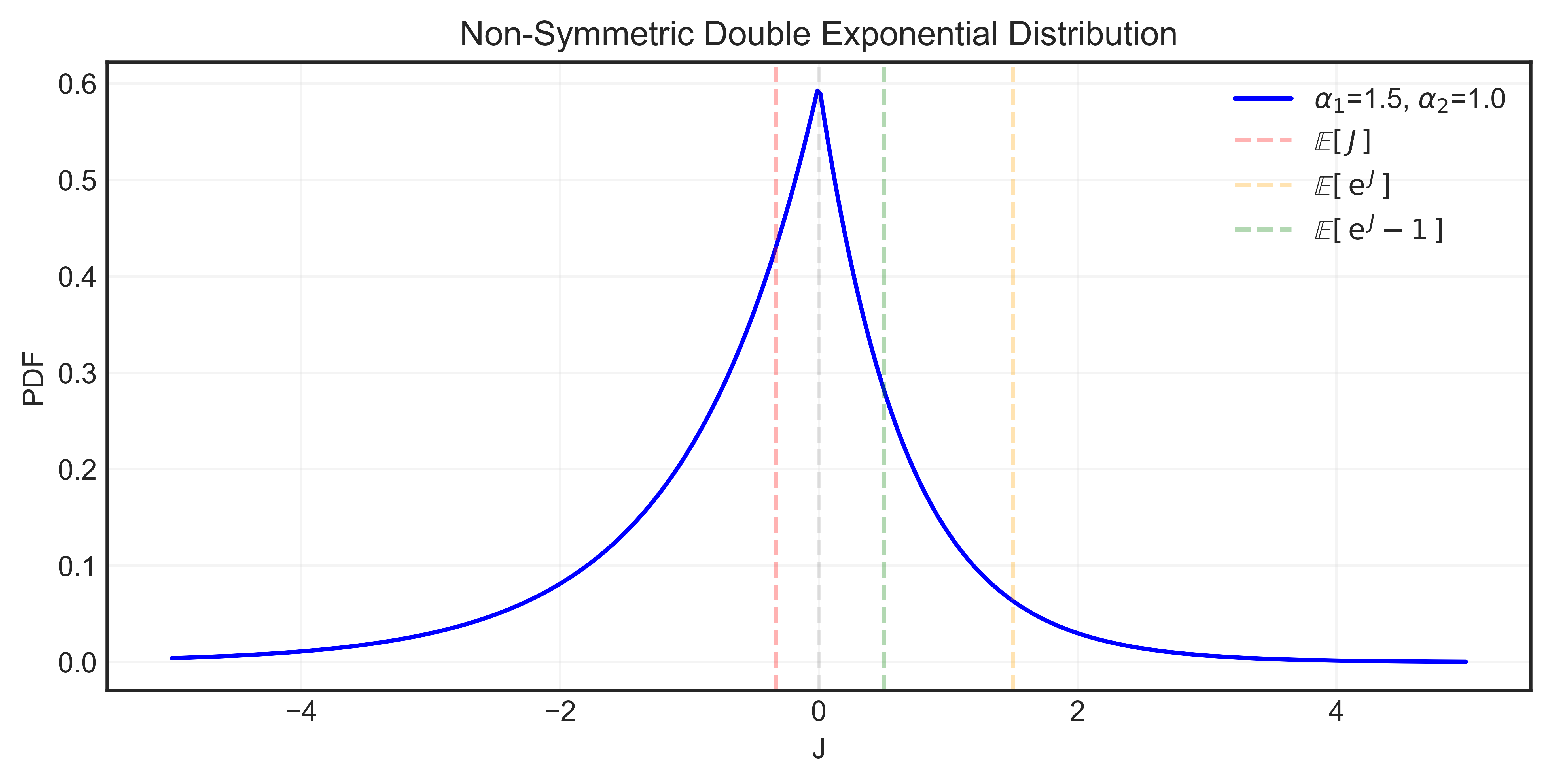 Figure 2. Non-symmetric double exponential distribution.
1
2
3
4
5
6
7
8
9
10
11
12
13
14
15
16
17
18
19
20
21
22
23
24
25
26
27
28
29
30
31
32
33
34
35
36
37
38
39
40
41
42
43
44
45
46
47
48
49
50
51
52
53
54
def nonsymmetric_double_exponential(x, alpha1, alpha2, p1, p2, plot=False):
    """
    Compute the PDF of the non-symmetric
    double exponential distribution and optionally plots it

    Input: alpha1 -> right tail decay rate
           alpha2 -> left tail decay rate
           normalization parameters p1, p2 with p1+p2 = 1
           random variable range x
    """
    pdf = np.where(
        x >= 0,
        p1 * alpha1 * np.exp(-alpha1 * x),  # Right tail (x >= 0)
        p2 * alpha2 * np.exp(alpha2 * x)    # Left tail (x < 0)
    )

    expected_val = (p1/alpha1) - p2/alpha2
    expected_jump = (p1 * alpha1/ (alpha1 - 1)) + (p2 * alpha2/ (alpha2 + 1))
    expected_jump_return = expected_jump - 1

    if plot:
        plt.figure(figsize=(9, 4))
        plt.plot(x, pdf, label= r"$\alpha_1$=" + f"{alpha1}, "
                 + r"$\alpha_2$=" + f"{alpha2}", color='b')

        plt.axvline(0, color='k', linestyle='--', alpha=0.1)  # Mark x = 0

        plt.axvline(expected_val, color='r', linestyle='--', alpha=0.3,
                    label = r"$\mathbb{E}\left[\,J\,\right]$")
        plt.axvline(expected_jump, color='orange', linestyle='--', alpha=0.3,
                    label = r"$\mathbb{E}\left[\,\mathrm{e}^{\,J}\,\right]$")
        plt.axvline(expected_jump_return, color='green', linestyle='--', alpha=0.3,
                    label = r"$\mathbb{E}\left[\,\mathrm{e}^{\,J} - 1\,\right]$")

        plt.xlabel("J")
        plt.ylabel("PDF")
        plt.title("Non-Symmetric Double Exponential Distribution")
        plt.legend()
        plt.grid(alpha=0.2)
        plt.show()

    return pdf

# Parameters
alpha1 = 1.5  # Decay rate for x >= 0
alpha2 = 1.0  # Decay rate for x < 0
p1 = alpha2 / (alpha1 + alpha2)  # Ensuring normalization
p2 = alpha1 / (alpha1 + alpha2)  # Ensuring normalization

# Generate x values
x = np.linspace(-5, 5, 400)

# Compute PDF values and plot
pdf = nonsymmetric_double_exponential(x, alpha1, alpha2, p1, p2, plot=True)