Intro to Jump Diffusion Models
I explore jump diffusion models that attempt to improve the shortcomings of Black Scholes pricing theory.
In a previous post, we took some conceptual steps away from the Black-Scholes pricing theory to motivate ourselves why in fact we might need to do so in order to appropriately take into account rare but extreme events such as market crashes. The presence of such events – which in fact constitute a type of market risk– in the market is expected to influence the prices of derivative contracts such as European vanilla options. When we consider the possibility of discontinuous jumps in the stock prices, we saw that we can no longer stay in the perfect risk-neutral world where a unique arbitrage-free price for securities exist. Instead, in the jumpy world, risk preferences of market participants re-enter back to the pricing framework, according to how likely an investor see the likelihood of jumps.
In this post, I will provide an introduction to jump-diffusion models that aim to capture jumpy nature of the stock’s along with the diffusive part described by standard Ito process.
To remind ourselves more explicitly the motivations for considering models that incorporate discontinuous jumps:
- The main appeal in jump-diffusion models is that observed stock prices do exhibit both upward and downward jumps. From the perspective of risk management, we would be more interested in the downside jumps which are pronounced at times of financial crisis such as the recent one in 2008. Furthermore, jump models provide a realistic framework for pricing options close to maturity as such options always have the possibility of entering out of money/ in the money zone in the presence of jumps.
- Jump-diffusion models extend the Black-Scholes pricing theory of options by introducing heavy tails (e.g. through extreme, rare events) and skinny shoulders (fewer moderate size returns) to return densities (e.g. log-returns with high kurtosis) which are an observed property of the stock (log) returns.
- By introducing a new modeling parameters to control the kurtosis and the asymmetry of the (log) stock return density, jump-diffusion models is able to capture the observed smile in the implied volatility.
Jump diffusion processes
Suppose that stock price $S(t)$ evolves under geometric Brownian Motion (GBM), along with the possibility of market crashes. What properties we expect the crashes to have? First, we expect these events to be rare. On the other hand, they should occur instantaneously such that the probability of occurrence within a time interval should be proportional to the length of the interval. We can encapsulate these properties by modeling the market crashes/jumps by a Poisson process as the latter model the number of events occurring in a fixed time interval, with the assumption that events happen independently and at a constant average rate of occurrence.
Let $N(t)$ is a Poisson process (with a rate/intensity/frequency $\lambda$ of jumps) describing the number of jumps that occur between time $0$ and $t$ (or up to time $t$). Here, $N(t)$ is an integer valued function that is constant for a while (between jumps) and increments by one when the jumps occur. The probability that a $j$ number of jumps occur until time $t$ is given by (see Appendix A):
\[\mathbb{P}(N(t) = j) = \frac{(\lambda t)^j}{j!}\, \mathrm{e}^{-\lambda t}.\]For a time interval $\Delta t$ between $t$ and $t + \Delta t$, we are interested in the increment of the counting process $\Delta N(t) = N(t + \Delta t) - N(t)$, i.e. the number of jump that occur within a time range of length $\Delta t$. By definition the increment process is also Poisson distributed: $N(t + \Delta t) - N(t) \sim \textrm{Poisson}(\lambda \Delta t)$ and we have:
\[\mathbb{P}(N(t+\Delta t) - N(t) = j) = \mathbb{P}(\Delta N(t) = j) = \frac{(\lambda \Delta t)^j}{j!}\, \mathrm{e}^{-\lambda \Delta t}.\]For a short time interval $\Delta t \ll 1$, the process can be approximated by a Bernoulli process with a jump/no jump probability that are given by
\[\begin{align} \nonumber \mathbb{P}(\Delta N(t) = 0) &\simeq 1 - \lambda \Delta t + \mathcal{O}\left(\Delta t^2\right),\\ \mathbb{P}(\Delta N(t) = 1) &\simeq \lambda \Delta t + \mathcal{O}\left(\Delta t^2\right). \end{align}\]Therefore, the change in the counting process during time interval will be 1 with probability $\lambda \Delta t$ and 0 with probability $1 - \lambda \Delta t$. The expected value in the incremental counting process is then given by
\[\mathbb{E}[\Delta N(t)] = \lambda \Delta t.\]Considering the discretized version of the incremental Poisson process $\Delta N_i = N_i - N_{i-1} $ for a unit length of time, we have
\[\mathbb{E}[\Delta N_i] = \lambda,\quad\quad \Rightarrow \quad\quad \mathbb{E}[N_t] = \mathbb{E}\left[\sum_{i = 1}^{t} \Delta N_i\right] = \sum_{i = 1}^{t} \mathbb{E}[\Delta N_i] = \lambda\, t.\]In Figure 1., we illustrate the discrete paths generated by a Poisson process $\Delta N(t)$ and the corresponding compensated Poisson process $\Delta \tilde{N}(t) = \Delta N(t) - \lambda \Delta t$ for $\lambda = 0.5$. The latter is of course adjusted to have a vanishing expectation, and if fact can be shown to be a martingale.
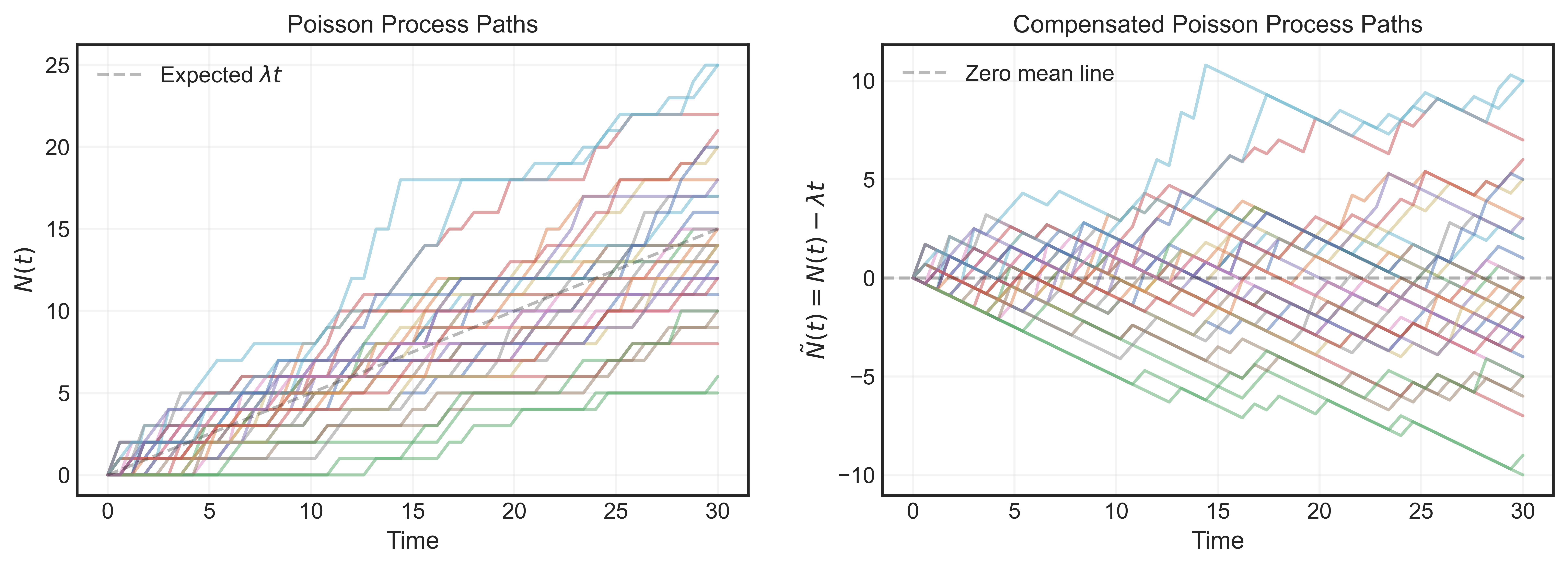 Figure 1. Monte Carlo simulation of Poisson process (left) and compensated Poisson process (right) paths.
Returning to the continuous process that describes the stock price, it is governed by the GBM superimposed with jumps. So we presume that when a jump occurs, the stock price becomes $S\,\mathrm{e}^J$ where $J$ is the jump magnitude which is itself a random variable. We could make a distributional assumption about $J$ or take it to be a single number. For now, we keep it as a general random variable. The process describing the stock price process can be therefore described as
\[\begin{equation}\label{jdp} \mathrm{d}S_t = \mu\, S_t\, \mathrm{d}t + \sigma\, S_t\, \mathrm{d}W_t + S_t (\mathrm{e}^J - 1)\, \mathrm{d}N_t. \end{equation}\]Note that when the jump occurs, the change in the stock price is $S (\mathrm{e}^J - 1)$ which is equivalent to multiplying the stock price with $\mathrm{e}^J$ after the jump. The exponential notation here is chosen carefully to restrict ourselves with positive stock prices after the jump. Here $J = 0$ corresponds to no jump and jump magnitudes with $0 > J > -\infty$ represents downward jumps and $J > 0$ is the domain for upward jumps. It is worth emphasizing that both the Wiener and Poisson process in \eqref{jdp} are defined under the real world probability measure, and they are assumed to be independent.
Given the jump-diffusion dynamics of the stock \eqref{jdp}, we should be able to price options. For example, we can try to find an equivalent martingale measure (equivalent to real world measure that governs \eqref{jdp}) and set the option prices to the discounted expectations of their pay-off in that measure, ensuring no arbitrage. Recall that the price we obtained in this way in just one of the many possible arbitrage-free prices as the market is incomplete in the presence of jumps. Essentially, as modeled by the last term in \eqref{jdp}, the number of possible jumps is a random variable within the timeline of the option contract, which in turn controlled by the intensity parameter $\lambda$ of the Poisson process. We therefore have an infinitely many risk-neutral measures parametrized by this parameter that characterize the “risk-aversiveness” of investors.
In analogy with Black-Scholes option pricing theory, another interesting question is: What is the partial differential equation that governs the option dynamics? Below, we will explore these issues. For this purpose, we will first digress a bit to train ourselves with the Ito calculus when the underlying stock follows a jump-diffusion process \eqref{jdp} we are focusing.
Ito-calculus in the presence of jumps. Consider a cadlag process consist of a drift and Poisson process:
\[\begin{equation}\label{cad} \mathrm{d}S_t = \bar{\mu}(t, S_t)\, \mathrm{d}t + \bar{J}(t, S_{t_{-}})\, \mathrm{d}N_t. \end{equation}\]where $\bar{\mu},\bar{J}$ are continuous functions. $S_{t_{-}}$ is the stock value just before the jump which can be defined as a limit of the stock price as we approach $t$ from the left:
\[S_{t_{-}} = \textrm{lim}_{s \to t_{-}} S_s.\]Similarly, $\bar{J}(t, S_{t_{-}})$ can be interpreted as the change in the stock value (determined by the stock value just before the jump) when a jump occurs $\mathrm{d}N_t = 1$, i.e. $S_t = S_{t_{-}} + \bar{J}(t,S_{t_{-}})$. As customary, we look for the process for a general function $f = f(t, S_t)$. Taylor expanding up-to second order we have the standard expression:
\[\begin{equation}\label{dfg} \mathrm{d}f(t, S_t) = \frac{\partial f}{\partial t}\, \mathrm{d}t + \frac{\partial f}{\partial S_t}\, \mathrm{d}S_t + \frac{1}{2} \frac{\partial^2 f}{\partial S_t^2}\, \mathrm{d}S_t^2. \end{equation}\]Unpacking all the terms above, we obtain:
\[\begin{align}\label{df} \mathrm{d}f(t, S_t) = \left( \frac{\partial f}{\partial t} + \bar{\mu} \frac{\partial f}{\partial S_t} \right)\,\mathrm{d}t + \bar{J} \frac{\partial f}{\partial S_t} \mathrm{d}N_t + \frac{1}{2}\left(\bar{\mu}\bar{J}\,\mathrm{d}t\,\mathrm{d}N_t + \bar{J}^2\,\mathrm{d}N_t^2\right) \frac{\partial^2 f}{\partial S_t^2}. \end{align}\]The last two terms are important here. Recall that as a rule of thumb we ignore terms that are $\mathcal{O}(\mathrm{d}t^2)$. First, inspecting the expectation of the cross term above,
\[\mathbb{E}[\mathrm{d}N_t \mathrm{d}t] = \mathrm{d}t \mathbb{E}[\mathrm{d}N_t] = \lambda \mathrm{d}t^2\]so we can ignore it to first order in short time increments $\mathrm{d}t$. On the other hand, notice that the squared Poisson process is equivalent to itself
\[\begin{equation} \mathrm{d}N_t^2 = \mathrm{d}N_t = \begin{cases} 1^2, \quad \textrm{with probability}\,\, \lambda \mathrm{d}t,\\ 0^2 \quad \textrm{with probability}\,\, 1 - \lambda \mathrm{d}t \end{cases} \end{equation}\]Implementing these findings in \eqref{df}, we obtain
\[\begin{equation}\label{df2} \mathrm{d}f(t, S_t) = \left( \frac{\partial f}{\partial t} + \bar{\mu} \frac{\partial f}{\partial S_t} \right)\,\mathrm{d}t + \left(\bar{J} \frac{\partial f}{\partial S_t} + \frac{1}{2} \bar{J}^2 \frac{\partial^2 f}{\partial S_t^2} \right)\mathrm{d}N_t \end{equation}\]Truncated to the second order in the $\bar{J}$ expansion, the square brackets in the last terms is essentially the difference of the process before and after the jump:
\[f(t,S_t) = f(t, S_{t_{-}} + \bar{J}(t,S_{t_{-}})) \simeq f(t, S_{t_{-}}) + \frac{\partial f}{\partial S_t} \bar{J} + \frac{1}{2} \frac{\partial^2 f}{\partial S_t^2} \bar{J}^2,\]which allow us to re-write \eqref{df2} as:
\[\begin{equation} \label{dfr} \mathrm{d}f(t, S_t) = \left( \frac{\partial f}{\partial t} + \bar{\mu} \frac{\partial f}{\partial S_t} \right)\,\mathrm{d}t + \left(f(t, S_{t_{-}} + \bar{J}(t,S_{t_{-}})) - f(t, S_{t_{-}})\right)\mathrm{d}N_t. \end{equation}\]We can generalize the result \eqref{dfr} by taking into account an additional diffusive term in the process \eqref{cad}:
\[\begin{equation}\label{jdpg} \mathrm{d} S_t=\bar{\mu}(t, S_t) \mathrm{d} t+ \bar{\sigma}(t, S_t) \mathrm{d} W_t + \bar{J}(t, S_{t_{-}}) \mathrm{d} N_t. \end{equation}\]Recalling the quadratic term in the stock price process in eq. \eqref{dfg}, we know from Ito’s lemma that $\mathrm{d} W_t^2 \to \mathrm{d} t$ and $\mathrm{d} W_t \mathrm{d}t \to 0$. On the other hand, there is an additional cross term of the form $\mathrm{d} W_t \mathrm{d}N_t$ we need to take into account which in fact has vanishing expectation due to the fact that diffusive process is independent of the Poisson process and the former has zero mean.
If the stock $S_t$ follows a jump-diffusion process of eq. \eqref{jdpg}, the process $df(t,S_t)$ thus satisfies
\[\begin{align} \nonumber \mathrm{d}f(t, S_t) = \left( \frac{\partial f}{\partial t} + \bar{\mu} \frac{\partial f}{\partial S_t} + \frac{\bar{\sigma}^2}{2} \frac{\partial^2 f}{\partial S_t^2}\right)\,\mathrm{d}t &+ \bar{\sigma} \frac{\partial f}{\partial S_t}\, \mathrm{d}W_t\\ &\quad\quad + \left(f(t, S_{t_{-}} + \bar{J}(t,S_{t_{-}})) - f(t, S_{t_{-}})\right)\,\mathrm{d}N_t.\label{ito} \end{align}\]This relation will be particularly handy for the derivation of the option dynamics when the underlying follows a jump-diffusion process. This is what we turn next.
Option dynamics in a jumpy world
Thus far, we focused on the stock dynamics in the real world measure, see e.g eq. \eqref{jdp}. To price the option in an arbitrage free manner, we need to derive its dynamics in the risk-neutral measure $\mathbb{Q}$. For this purpose, we need to determine the condition under which the discounted stock price \(\tilde{S}_{t} = S_{t} / Z_{t}\) is a Martingale.
Here, $Z_t$ is a zero coupon bond (or money market account) that has a deterministic dynamics $\mathrm{d}Z_t = r\, Z_t\, \mathrm{d}t$. If \(\tilde{S}_t\) is a Martingale, then the increment process \(\mathrm{d}\tilde{S}_t = \tilde{S}_{t + \mathrm{d}t} - \tilde{S}_t\) should have a zero conditional expectation under the filtration $\mathcal{F}_t$:
\[\begin{equation}\label{mc} \mathbb{E}\left[\mathrm{d}\tilde{S}_t | \mathcal{F}_t\right] = 0, \quad\quad \mathrm{d}\tilde{S}_t \equiv \tilde{S}_{t + \mathrm{d}t} - \tilde{S}_t = \frac{\mathrm{d}S_t}{Z_t} - r \frac{S_t}{Z_t} \mathrm{d}t. \end{equation}\]Inserting the stock dynamics \eqref{jdp} in the equation above, we obtain
\[\begin{equation}\label{mc2} Z_t \mathbb{E}\left[\mathrm{d}\tilde{S}_t | \mathcal{F}_t\right] = \mathbb{E}\left[\mu S_t -r S_t | \mathcal{F}_t\right] \mathrm{d} t + \mathbb{E}[\sigma S_t \mathrm{d} W_t | \mathcal{F}_t] + \mathbb{E}\left[\left(\mathrm{e}^J-1\right) S_t \mathrm{d} N_t | \mathcal{F}_t\right] = 0. \end{equation}\]In the expression above, stochastic quantities such as the stock price evaluated at $t$ can be taken outside the integral due to the conditioning on the filtration. Furthermore, since the Brownian motion $W_t$ is a Martingale, its increment have zero expectation, making the second term on the right-hand side vanishing. Finally, the random variable $J$ is assumed to be independent of the Poisson process, such that the expectation in the final term factorizes to give
\[\mathbb{E}\left[\left(\mathrm{e}^J-1\right) S_t\, \mathrm{d} N_t | \mathcal{F}_t\right] = S_t\, \mathbb{E}\left[\mathrm{e}^J-1\right] \mathbb{E}\left[\mathrm{d}N_t\right] = \lambda\, S_t\, \mathbb{E}\left[\mathrm{e}^J-1\right] \mathrm{d}t.\]Applied to \eqref{mc2}, all this information gives us
\[\mathbb{E}\left[\mu S_t -r S_t | \mathcal{F}_t\right] \mathrm{d} t + \lambda\, S_t\, \mathbb{E}\left[\mathrm{e}^J-1\right] \mathrm{d}t = 0 \quad \Longrightarrow \quad (\mu - r + \lambda \mathbb{E}\left[\mathrm{e}^J-1\right]) S_t \mathrm{d}t = 0.\]This relation gives us the drift the stock price must obey under the risk neutral measure $\mathbb{Q}$:
\[\begin{equation}\label{rnd} \mu = r - \lambda \mathbb{E}\left[\mathrm{e}^J-1\right], \end{equation}\]and the dynamics of the stock under this measure is given by
\[\frac{\mathrm{d}S_t}{S_t} = (r - \lambda \mathbb{E}\left[\mathrm{e}^J-1\right])\mathrm{d}t + \sigma\,\mathrm{d}W^{\mathbb{Q}}_t + (\mathrm{e}^J - 1)\, \mathrm{d}N_t.\]We can then find an arbitrage-free price for a European option $O$ with maturity $T$ through the risk-neutral expectation of its discounted pay-off:
\[\begin{equation}\label{rop} \frac{O_t(S_t)}{Z_t} = \mathbb{E}_{\mathbb{Q}}\left[\frac{O_T(S_T)}{Z_T} \bigg |\, \mathcal{F}_t\right]. \end{equation}\]Before we get there we can utilize the same trick we applied for the stock evolution to derive the dynamics of the option under the risk-neutral measure. For this purpose, we use the fact that $O_t/Z_t$ in \eqref{rop} is a Martingale under the risk-neutral measure $\mathbb{Q}$, so that its incremental process has zero mean under the same measure:
\[\begin{equation}\label{odr} \mathbb{E}_{\mathbb{Q}}\left[\mathrm{d}\left(\frac{O_t(S_t)}{Z_t}\right) \bigg| \mathcal{F}_t\right] = 0,\quad\quad \mathrm{d}\left(\frac{O_t}{Z_t}\right) = \frac{\mathrm{d}O_t}{Z_t} - r \frac{O_t}{Z_t}\,\mathrm{d}t. \end{equation}\]Using the Ito’s lemma we found for a jump diffusion process in eq. \eqref{ito}, we identify $f(t,S_t) = O_t$ and $\bar{J} = (\mathrm{e}^J - 1) S_t$, we have
\[\begin{align} \nonumber \mathrm{d}\left(\frac{O_t}{Z_t}\right) &= \frac{1}{Z_t} \left(\frac{\partial O_t (S_t)}{\partial t} + \bar{\mu}(t, S_t) \frac{\partial O_t (S_t)}{\partial S_t} + \frac{\bar{\sigma}^2(t,S_t)}{2} \frac{\partial^2 O_t(S_t)}{\partial S_t^2} - r O_t(S_t)\right) \mathrm{d}t\\ &\quad\quad\quad\quad\quad\quad\quad\quad\quad\quad + \frac{\bar{\sigma}(t,S_t)}{Z_t} \frac{\partial O_t(S_t)}{\partial S_t}\, \mathrm{d}W_t^{\mathbb{Q}} + Z_t^{-1} \left(O_t(S_t \mathrm{e}^J) - O_t(S_t)\right)\,\mathrm{d}N_t.\label{dm} \end{align}\]Plugged in the expectation in \eqref{odr}, the diffusive term ($\propto \mathrm{d}W_t^{\mathbb{Q}}$) in \eqref{dm} is vanishing, we then note again the independence of jumps and the Poisson process, to obtain
\[\begin{align} &\nonumber\left(\frac{\partial O_t (S_t)}{\partial t} + \bar{\mu}(t, S_t) \frac{\partial O_t (S_t)}{\partial S_t} + \frac{\bar{\sigma}^2(t,S_t)}{2} \frac{\partial^2 O_t(S_t)}{\partial S_t^2} - r O_t(S_t)\right)\, \mathrm{d}t\\ &\quad\quad\quad\quad\quad\quad\quad\quad\quad\quad\quad + \mathbb{E}_{\mathbb{Q}}[(O_t(S_t \mathrm{e}^J)- O_t(S_t)) | \mathcal{F}_t]\, \mathbb{E}_{\mathbb{Q}}[\mathrm{d}N_t\, |\, \mathcal{F}_t] = 0 \end{align}\]Evaluating the last expectation, we note the risk-neutral drift $\bar{\mu} = \mu S_t$ with $\mu$ given by \eqref{rnd} and $\bar{\sigma} = \sigma S_t$ to finally obtain the pricing equation as:
\[\begin{align} \nonumber \frac{\partial O_t (S_t)}{\partial t} &+ (r - \lambda \mathbb{E}\left[\mathrm{e}^J-1\right]) S_t \frac{\partial O_t (S_t)}{\partial S_t} + \frac{\sigma^2 S_t^2}{2} \frac{\partial^2 O_t(S_t)}{\partial S_t^2}\\ &\quad\quad\quad\quad\quad\quad\quad\quad\quad\quad\quad\quad\quad - (r + \lambda) O_t(S_t) + \lambda \mathbb{E}_{\mathbb{Q}}[O_t(S_t \mathrm{e}^J) | \mathcal{F}_t] = 0. \end{align}\]Due to the presence of the expectation (over the distribution of jumps $J$), this is a partial integro-differential equation (PIDE) which reduces to the Black-Scholes PDE in the $\lambda \to 0$ limit as expected. PIDEs are typically more difficult to solve as compared to PDEs due to the presence of the additional integral term. For only a handful of models that in fact make simplifying assumptions about the distribution of $J$, analytic solutions exist. In this context, I will focus on a simple alternative route to derive a closed form solution in another post.
References
1. “The concepts and practice of mathematical finance”, Second Edition, Mark S. Joshi.
2. “Volatility and Correlation: The perfect hedger and the fox”, Second Edition, Riccardo Rebonato.
3. “Mathematical Modeling and Computation in Finance”, World Scientific, Cornelis W. Oosterlee and Lech A. Grzelak.
Appendix A: Poisson distribution and process
The Poisson distribution is a discrete probability distribution that expresses the probability of a given number of events occurring in a fixed interval of time if these events occur with a known constant mean rate $\lambda$ (e.g. average number of calls a call center receive in a minute) and independently of the time since the last event. A Poisson random variable which we denote by $N$,counts the number of occurrences of an event during a given (fixed) time period. The probability of observing $k\geq 0$ occurrences within the time period is given by the following pmf:
\[\begin{equation} \mathbb{P}(N = k) = \frac{\lambda^k}{k!} \mathrm{e}^{-\lambda}. \end{equation}\]By definition the expected number of occurrence of the event is given by $\mathbb{E}[N] = \lambda$ and noting
\[\begin{align} \nonumber \mathrm{e}^{-\lambda}\, \lambda^2 \frac{\partial^2}{\partial\lambda^2} \left(\sum_{k = 0}^{\infty} \frac{\lambda^k}{k!}\right) &= \lambda^2,\\ \mathrm{e}^{-\lambda} \sum_{k = 0}^{\infty} k\,(k - 1) \frac{\lambda^k}{k!} &= \mathbb{E}[N^2] - \mathbb{E}[N], \end{align}\]its variance is given by
\[\mathbb{E}[N^2] = \lambda^2 + \lambda \quad \Rightarrow \quad \mathbb{V}[N] = \mathbb{E}[N^2] - \mathbb{E}[N]^2 = (\lambda^2 + \lambda) - \lambda^2 = \lambda.\]We denote $N \sim \textrm{Poisson}(\lambda)$ to emphasize that the variable $N$ has a Poisson distribution with parameter $\lambda$. Now, if we want to track dynamically the number of occurrence of events over time (e.g. in a cumulative sense) instead of a single fixed time interval, Poisson process provides a suitable generalization by allowing us to track how these events happen over continuous time.
Poisson Process. A Poisson process ${N(t),\,t\geq 0}$ with parameter $\lambda$ is an integer valued stochastic process with the following properties
- $N(0) = 0$
- $\forall t_0 = 0 < t_1 < t_2 < \dots < t_n $, the increments of the process $N(t_1) - N(t_0), N(t_2) - N(t_1), \dots, N(t_n) - N(t_{n-1})$ are all independent random variables.
- for $s \geq 0$ and $t > 0$, and integers $k \geq 0$, the increments are Poisson distributed:
where $\lambda$ is the rate/intensity of the Poisson process. The process $N(t)$, which counts the number of events between times $0$ and $t$ (e.g. $s = 0$ in eq. \eqref{ppd}), is a counting process with the number of events in any time period of length $t$ is specified through eq. \eqref{ppd}. The eq. \eqref{ppd} also implies that the increments are stationary in the sense that statistical properties of the increments do only depend on the length of the interval and not on the starting time of the increment. In other words, the process do not have a memory of where you start counting the number of events, only the length of time interval matters.
Appendix B: Python code for Monte-Carlo simulation of Poisson Process
Using the helper function defined below, we generate paths for the Poisson process with a given intensity $\lambda$.
1
2
3
4
5
6
7
8
9
10
11
12
13
14
15
16
17
18
19
20
21
22
23
24
25
26
27
28
29
30
31
32
33
34
35
36
37
38
39
40
41
42
43
44
45
46
47
48
49
50
51
52
53
54
55
56
57
58
59
60
61
62
63
64
65
66
67
import pandas as pd
import numpy as np
import seaborn as sns
import matplotlib.pyplot as plt


#For inline plotting
%matplotlib inline
%config InlineBackend.figure_format = 'svg'

# set plot properties to seaborn globally
plt.style.use("seaborn-v0_8-white")

def generate_poisson_paths(T, num_time_steps, lmbd, num_sim = 1, plot = True):

    '''
    Helper function to simulate & plot Poisson process paths

    ### Inputs
    num_sim: number of paths to simulate
    T: total time span of each simulation
    num_time_steps: number of time steps to simulate the paths
    lmbd: rate/intensity of poisson process
    plot: default to True

    ### Output: tuple
    time span of the sims, Poisson process paths and compensated process
    '''

    dt = T / num_time_steps  # Time step size
    times = np.linspace(0, T, num_time_steps + 1)  # Time grid

    # Generate Poisson-distributed increments in a vectorized manner
    increments = np.random.poisson(lmbd * dt, size=(num_sim, num_time_steps))

    # Compute Poisson paths using cumulative sum (vectorized)
    N_paths = np.zeros((num_sim, num_time_steps + 1))
    N_paths[:, 1:] = np.cumsum(increments, axis=1)

    # Compute compensated Poisson process
    N_tilde_paths = N_paths - lmbd * times  # N(t) - λt

    # Plot results
    if plot:

        _ , axes = plt.subplots(1,2, figsize = (13,4))

        axes[0].plot(times, N_paths.T, alpha=0.5)
        axes[0].plot(times, lmbd * times, 'k--', label=r'Expected $\lambda t$', alpha = 0.3)
        axes[0].set_xlabel('Time')
        axes[0].set_ylabel(r'$N(t)$')
        axes[0].set_title('Poisson Process Paths')
        axes[0].grid(alpha = 0.2)
        axes[0].legend()

        axes[1].plot(times, N_tilde_paths.T, alpha=0.5)
        axes[1].axhline(0, color='k', linestyle='--', label='Zero mean line', alpha = 0.3)
        axes[1].set_xlabel('Time')
        axes[1].set_ylabel(r'$\tilde{N}(t) = N(t) - \lambda t$')
        axes[1].set_title('Compensated Poisson Process Paths')
        axes[1].grid(alpha = 0.2)
        axes[1].legend()

    return times, N_paths, N_tilde_paths

# Call the function to plot
time_grid, poisson_sim, comp_poisson_sim = generate_poisson_paths(30,50,0.5, num_sim = 35)