Above and Beyond Black-Scholes world

In a series of earlier posts, I covered Black-Scholes option pricing theory. There, we saw that assuming risk-neutrality of investors lead to a unique arbitrage-free price for European type options. In fact, assuming log-normality of the underlying stock price, we were able to derive a simple analytic formula that describes this price in terms a few parameters that characterize the contract (e.g. time to maturity $T$, strike $K$), as well as market observables (e.g. risk-free rate $r$ and spot $S$). In all these derivations, several concepts such as hedging and risk-neutrality of the investors appeared in a rather convoluted way. Another concept called the replicating portfolio appeared less so. I Therefore, I would like to start this post by an attempt to clarify the role played by these concepts for pricing options, putting an emphasis on the pricing with replication. To make the discussion intuitive, first I will focus on simple single (time) step binomial tree as shown in Figure 1.

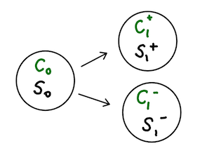Figure 1. Single time step binomial model for option pricing.

In this world, we are interested in pricing a call option $C_0$ today ($t = 0$) given we have the information about the spot price $S_0$. Tomorrow, we assume that the stock price can take up two possible values, corresponding to a small up/down move $S_1^{\pm}$. We assume that the call option has a strike $K$ that satisfies $S_1^{+} > K > S_1^{-} $ so that it will certainly be exercised at $t = 1$ with a value of $C_1^{+} = S_1^{+} - K$ in the up branch, otherwise expires with a vanishing value $C_1^{-} = 0$. To further simplify the discussion we will take the risk-free rate as $r = 0$, to ensure the presence of a third asset in the market: a zero coupon bond (or money market account) that takes $B_0 = 1$ and $B_1 = 1$ at both time steps. Without loss of generality, we take $S_0 = 100$, $K = 100$, $S^{+}_1 = 110$ and $S^{-}_1 = 90$ which implies $C_1^{+} = 10$ and $C_1^{-} = 0$.

Pricing with Hedging. Assume that we are an option dealer, when we sell a call option we are exposed to a type of market risk (more specifically delta risk) that the stock price may rise above the strike. To simply protect ourselves, we can extend our portfolio to buy a fixed $\Delta$ amount of stock: $V = \Delta S - C$. We are still not perfectly hedged as the portfolio can still take up two different values depending on the two states of the world as shown in Figure 1. Complete hedging in our world simply means to remove all the uncertainty associated with the $\pm$ states of tomorrow:

\[\begin{equation}\label{D} \Delta S_1^{+} - C_1^{+} = \Delta S_1^{-} - C_1^{-}\quad\quad \Longrightarrow \quad\quad \Delta = 1/2. \end{equation}\]

This result implies that if we buy half a stock, our portfolio is worth the same $V_1^{\pm} = 45$ in every state of the world tomorrow which is equivalent to 45 riskless bond tomorrow. Since we assume $r = 0$, it must therefore be worth the same today $V_0 = V_1^{\pm} = 45$, otherwise there are arbitrage opportunities: e.g. if $V_0 < 45 $, we can borrow $V_0$ amount from the bank and immediately invest on the portfolio which is guaranteed to become $V_1 = 45$ tomorrow. We can pay back our loan and pocket the risk-free amount of $V_1 - V_0 > 0$.

Therefore, hedging our short position in the call option with a Delta amount of stock lead to arbitrage free portfolio which in turn enforces the price of the call option $C_0$:

\[V_0 = \Delta S_0 - C_0 \quad\quad \Longrightarrow \quad\quad C_0 = \Delta S_0 - V_0 = \frac{100}{2} - 45 = 5.\]

Risk-neutral pricing. In this framework, we think in terms of probabilities of the up $p_+$ and down $p_{-} = 1 - p_{+}$ move of the stock price tomorrow. To ensure no-arbitrage in our simple two state world, it is enough to have non-zero probabilities for both states, i.e. $0 < p_+ < 1$, simply because the stock cannot grow faster than the risk-free-rate. In other words, the role of the probabilities is to ensure both states are possible which ensures no-arbitrage. Now, we ask ourselves the question, if we buy the stock today, how much minimum return should we require tomorrow over the risk-free money market account? Instead of investing on a risky stock, I can always put $S_0$ amount in the bank which becomes $S_0\,\mathrm{e}^{r \delta t}$ tomorrow and I make risk-free $S_0 \,\mathrm{e}^{r \delta t} - S_0$ amount. Therefore, the least I can expect from the stock is to perform as if I invest the $S_0$ amount in the money market:

\[\mathbb{E}[S_1] = S_0\, \mathrm{e}^{r \delta t} \quad\quad \xrightarrow{r = 0} \quad\quad \mathbb{E}[S_1] = S_0.\]

For our special world with $r = 0$, this implies that best I can expect from the stock price tomorrow is just its price today and nothing else. The relation above sets the main ideology in this framework: the investors are risk-neutral in the sense that by investing into the stock, we do not expect extra reward for the riskiness of the stock over a risk-free bond. Risk-neutrality then give rise to the risk-neutral probabilities via:

\[\begin{equation}\label{rnp} \mathbb{E}[S_1] = p_+ S_1^{+} + (1-p_+) S_1^{-} = S_0 \quad\quad \Longrightarrow \quad\quad p_+ = \frac{S_0 - S_1^{-}}{S_1^+ - S_1^-} = \frac{1}{2}. \end{equation}\]

Therefore, the risk-neutral world assign equal probabilities for the up/down moves of the stock price. Similarly, this probability sets the fair price of a game with two possible outcomes $C_1^{\pm}$:

\[\mathbb{E}[C_1] = C_0\, \mathrm{e}^{r \delta t} \quad\quad \xrightarrow{r = 0} \quad\quad \mathbb{E}[C_1] = C_0 = p_+ C_1^{+} = 5,\]

which is equivalent to the arbitrage-free price based on the hedging argument above. In other words, risk-neutrality point to a unique arbitrage free price! In reality, investors tend to be more risk-averse than risk-neutral, which implies $p_+ > 1/2$.

Pricing by replication. The replication method relies on a rather simple idea which simply states that the price of the option is the cost of a portfolio that replicates the options pay-off at the maturity. In other words, if we can construct a portfolio that replicates the option’s pay-off in all possible states of the world tomorrow, the price of the option must therefore agree with that portfolio’s value, otherwise there would be arbitrage. Not surprisingly one can construct such a portfolio in terms of the stock and bonds. The slope of this portfolio will correspond to the amount of stock we must hold whereas the intercept (at $S = 0$) will correspond to the amount of bonds.

To illustrate this, consider a general European type option that is either $C_1^{+} = \alpha + \beta$ or $C_1^{-} = \alpha$ at the maturity. We sold this option and collected a fee $C_0$. Our replicating portfolio must satisfy $b S_1 + a = C_1$. In our two state world, we need to just solve a linear system of equations with 2 unknowns:

\[\begin{align} \nonumber 110\, b + a &= \alpha + \beta,\\ 90\,b + a &= \alpha. \end{align}\]

Subtracting them gives $b = \beta / 20$ which we use to obtain the amount of bonds that we need to hold as $a = \alpha - 4.5 \beta$. Then the value of the portfolio today must agree with the option price $C_0$:

\[\begin{equation}\label{prep} V_0 = C_0 = \frac{\beta}{20} S_0 + (\alpha - 4.5 \beta) = 0.5 \beta + \alpha. \end{equation}\]

Here, we worked intentionally with an arbitrary European type option that has a determined pay-off in order to essentially emphasize the breadth of applicability of the replication idea. For the call option (struck at $K = 100$) we have been working so far, we have $C_1^{-} = \alpha = 0$ and so $C_1^{+} = \alpha + \beta = \beta = 10$, and so, in eq. \eqref{prep}, we again get the same unique price implied by the hedging and risk-neutrality arguments, i.e. $C_0 = 5$. Notice that the amount of stock we must hold in the replicating portfolio, i.e $\beta / 20 = 1/2$ is the same as the amount implied by the hedging arguments, see eq. \eqref{D}.

To summarize, in this framework, the price of an option is thus the sum of money, which by being invested appropriately today, is guaranteed to match the option’s pay-off in all possible states of the world tomorrow!

A three state world: towards incomplete markets

---

At this point, our two state model appears to be an oversimplification. There is certainly room for other states for the value of an asset. One possibility is to include a downward jump of certain size in the stock price, which could be helpful to parametrize shocks in the stock market. This direction is in fact where this post is aiming at. However, before we get there we can think of even milder situations to study the implications of more than two states. For this purpose we will consider a third state $S_1^{(0)} = 100$ for tomorrow and again we would like to price a call option with strike $K = 100$.

Using hedging arguments, we should decide the amount $\gamma$ of stock we should by to hedge our position in the call option for this three state world. Our portfolio $\gamma S - C$ has the following possible values at the maturity:

\[\begin{align} \nonumber V_1^{+} &= \gamma S_1^{+} - C_1^{+} = 110 \gamma - 10,\\ \nonumber V_1^{(0)} &= \gamma S_1^{(0)} - C_1^{(0)} = 100 \gamma,\\ V_1^{-} &= \gamma S_1^{-} - C_1^{-} = 90 \gamma. \end{align}\]

There are three equations with one unknown, so there is no unique solution as before. For example, if we equate the last two equations, we get $\gamma = 0$, we get $V_1^{+} = -10$ and $V_1^{(0)} = V_1^{-} = 0$, so we are not hedged at all! Another option would be to ignore the $(0)$ state and hedge the portfolio implied by the $\pm$ states, which implies $\gamma = 1/2$ as before with $V_1^{\pm} = 45$ and $V_1^{(0)} = 50$. Now, we are hedged partially but our portfolio does have some variability tomorrow, i.e our portfolio is not completely risk-free. However, in this case we know that it must worth at least 45 tomorrow and possibly more, so it can today by arbitrage arguments:

\[V_0 = \gamma S_0 - C_0 \geq 45 \quad\quad \Longrightarrow \quad\quad C_0 \leq 5.\]

Therefore, the best we can do is to put an upper bound on the options price. If we were to apply pricing with replication, notice that we would get three equations with two unknowns parametrized by the amount of stock and bonds that the replicating portfolio must include. The system is over determined and so there is no unique portfolio that replicates the option’s pay-off but rather one can find a portfolio that dominates the pay-off of the option at all three states at the maturity, consistent with our finding above.

It is also instructive to have a look at risk-neutral valuation in this three state world. In this world, investors do not expect extra rewards from risky assets, at least not more than the investments on riskless bonds and so \(\mathbb{E}[S_1] = S_0\). To satisfy this relation, we can assume an equall up and down risk-netural probability $p_+ = p_{-}$ corresponding to the probability $p_0 = 1 - 2p_+$ of the neutral state. In this case we see that there is an infinite set of probability measures that satisfies the condition as long as $p_+ \in (0,1/2]$ to avoid any zero probability for the $\pm$ states. To see this notice that for these choices of probability, risk-neutrality condition is automatically satisfied:

\[\mathbb{E}[S_1] = 200 p_+ + (1 - 2 p_+) 100 = 100.\]

Then the risk-neutral price of the option is determined via:

\[\mathbb{E}[C_1] = C_0 = 10 p_+ \,\in\, (0,5]\]

same as implied by the hedging argument above. In other words, the risk-neutrality implies that prices that satisfy $0 < C_0 \leq 5$ are not arbitrageable.

The presence of the third state brings us to the concept of an incomplete market. In incomplete markets, an arbitrary pay-off of a European contingent claim can not be precisely replicated by a self-financing portfolio/trading strategy. As a result, it is a characteristic property of incomplete markets that the price of an option can only be bounded rather than being forced to take a unique value.

Remark. Incomplete markets take us away from the perfect risk-neutral world of Black-Scholes in that the market price of such an option will be within a range of possible prices determined by the risk-preferences of the investors in the market rather than mathematical framework of risk-neutrality.

One may wonder if we can complete the market in some way and another related question is what it takes to complete the market? Below I will briefly dwell into these issues following Rebonato’s book.

From the perspective of the replication argument for the single step tree above, the issue is clear: we have two unknowns corresponding to the holdings of 2 assets (stocks and bonds) used for the replication, but we have three equations representing the value of the option we are trying to replicate in all three states of the world tomorrow. A simple solution we may consider is therefore to add another instrument that can be used in the replicating portfolio. Why not use a hedging option (say a call option), stocks and bonds to replicate another call option on the same underlying. Parametrized by the 3 probable values the stock might take, we thus consider to include a “hedging” call option struck at $K_1$, so that $C_1(t = 1) = \textrm{max}(S_i - K_1, 0)$ to replicate another struck at $K_2$ with the following pay-off $C_2(t=1) = \textrm{max}(S_i - K_2, 0)$ where $i = \pm, j$ represents the states of the world tomorrow. The portfolio we construct (at $t = 0$) with these instruments must replicate the second option’s pay-off (at $t = 1$), so the following linear system must hold

\[\begin{align} \begin{bmatrix} S^{+} & B^{+} & C_1^{+} \\ S^{-} & B^{-} & C_1^{-} \\ S^{j} & B^{j} & C_1^{j} \end{bmatrix}\, \begin{bmatrix} a \\ b \\ c \end{bmatrix} = \begin{bmatrix} C_2^{+} \\ C_2^{-}\\ C_2^{j} \end{bmatrix} \end{align}\]

which has the ${\bf S} \vec{x} = \vec{y}$. As longs as the “state” matrix ${\bf S}$ is invertible – which holds almost surely as the columns are linearly independent – , we can then solve for the holdings vector to get $\vec{x} = [\,a\,\, b\,\, c\,]^T$. Since the value of this portfolio is worth as much as the option $C_2$ at the pay-off its value must also agree today by arbitrage considerations:

\[C_2(0) = \hat{a}\, S(0) + \hat{b}\, B(0) + \hat{c}\, C_1(0).\]

In fact, as far as we deal with one period option to be replicated (or equivalently hedged) with one period options of different strikes, we can extend the analysis above to more complex situations that involve $2,3,\dots,n$ possible jump amplitudes. For example, for $n$ possible jump amplitudes, on top of stocks and bonds, we would need $n$ additional options to complete the market. In this case, we would just to solve a $(n + 2) \times (n+2)$ system of linear equations to uniquely determined the holding of the replicating portfolio.

These results, when taken at face value, suggest that if only a finite number of jump amplitudes were possible, we could replicate an option using as many options as possible and as a result market participants would always agree with the price of the target option undoubtedly. In other words, our risk preferences would play no role in determining the price as the market appear to be complete. Stated in another way, we can think of the chosen jump amplitudes to produce a stock price distribution similar to the one generated by the pure diffusion case, i.e. a risk neutral measure. As a result, one would be tempted to conclude that in pricing all types of European options risk preferences of investors would likely to play a limited role even in the general case including random jump amplitudes!

These arguments based on the single step tree needs strong justifications. In fact, although mathematically things seem to work and the market is complete in this setting, it immediately breaks down in realistic setups with multiple time step trading horizon.

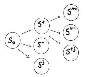Figure 2. Jumpy stock price process in two time steps. Only the states in the upper branch $+$ is shown.

Now consider a two time-step process in Figure 2 where we only show the process of the stock price in the upper branch. It should be noted that here we do not have the knowledge of the stock price at $t = 1$ and $t = 2$. All we are doing here is to label/parametrize the possible states without knowing the actual probabilities to reach that state. The options $C_1$ and $C_2$ are derived from the same underlying stock shown in the Figure and both expire at the final time step with a known pay-off in terms of the stock price. In this setup, it is immediately clear why we can not replicate the options pay-off as apart from the final states we show in the Figure 2., the stock exhibits three more unique states $S^{–}, S^{-j}, S^{jj}$ and the corresponding states for the target option $C_2(t = 2)$. We simply have three unknown holdings for the replicating portfolio and 6 equations which is again over-determined, so we are back to incomplete markets where we can not uniquely price $C_2$ and risk preferences of the investors are back in the picture.

What do we need to achieve a replicating portfolio? We could as well solve the $3 \times 3$ system of equations coming out of for each of the first states $+, -$ and $j$ to obtain the value of the replication portfolio in the last time step, then by no-arbitrage considerations we would have the target option’s value in the first time step which is encoded in the $C_2^{\pm}$ and $C_2^{j}$: this is a $3 \times 3$ system as well that can be solved. However the value of the portfolio now contains the value of the hedging option in all the future states, $C_1^{\pm}$ and $C_1^{j}$, which are not known to us from today’s prices. Therefore, from this perspective, we should know not just the price of the hedging option $C_1$ today but also its value in all future possible states of the world! This is why uniquely pricing contingent claims via replicating portfolio’s built by stocks, bonds and options, is not feasible in the real jumpy markets.

Pricing Options in incomplete markets

---

The arguments above have already showed us the fragility of the Black-Scholes model of pricing options which is essentially based on the concepts of risk neutrality, continuous hedging and no-arbitrage principle. There are further criticisms to the model which I would like to mention here:

• First, the standard treatment in the Black-Scholes (BS) model assumes a normal distribution of the underlying stock returns, which is unable to capture the fat tails observed seen in the historical stock price returns.
• Second, in the BS world asset prices are taken as continuous functions. For example, a continuous analytic form for the option price can be derived using multiple step binomial trees taking the limit of small step size in the time domain. However, the real world markets are known to exhibit shocks/abrupt corrections which lead to discontinuous downward movement in the asset prices making the perpetual re-hedging impractical during the lifetime of the option contract.

To obtain a better phenomenological model, we can modify it by adding such dramatic downward moves that has a particular size. This will of course take us into the realm of incomplete market: with three possible states, there is no unique arbitrage free price, independent of the number of time steps. For example, we can apply the risk-neutral valuation as above, and since there are infinitely many ways to distribute the probabilities consistent with risk-neutrality between the three nodes, no unique arbitrage free price exist! Consider for example the case we studied in Figure 1. by adding a third possibility of the stock jumping to $60$ tomorrow, and for $S_0 = 100$ we again wish to price a call option struck at $100$. Assigning the probabilities of each state tomorrow, we need to solve

\[110 p_u + 90 p_d + 60 p_j = 100\]

subject to $p_u + p_d + p_j = 1$. Solving for the probability of small up and down moves in terms of the probability of jump we get

\[\begin{align} \nonumber p_u &= \frac{1}{2} + \frac{3}{2} p_j,\\ p_d &= \frac{1}{2} - \frac{5}{2} p_j. \end{align}\]

So we have infinitely many risk-neutral measures parametrized by $p_j \in [0, 1/5]$. The price of the option struck at $K = 100$ can then be anywhere between 5 and $8$ without introducing arbitrage:

\[C_0 = \mathbb{E}[C_1] = 10 p_u = 5 + 15 p_j \, \in \, [5,8].\]

The exact choice of the price of the option is then simply a question related to risk-preferences or how risk-aversive one is.

One solution to obtain a unique price is to assume that the price jump probabilities $p_j$ to live in the real-world rather than the risk-neutral world and adjust the probabilities of the small up/down moves to obtain the unique risk-neutral probabilities consistent with it. Whilst this certainly allows us to obtain an arbitrage-free price, it is just one of the many possible arbitrage-free price. Models of this sort are known as jump-diffusion models, which are essentially a fusion of an underlying diffusive stochastic process consisting of small price fluctuations with that of a jumpy process.

From an empirical perspective, these models have some validity because stock prices are jumpy and that the volatility smiles of equity options (volatility implied by the option prices at different strikes) are certainly skewed – with high slopes (in absolute value) for low $K$ and small slopes at large $K$–, reflecting the fact that stock prices are much more likely to jump down then up. The skewness of the volatility smiles is also just a reflection of supply and demand dynamics where many investors have a tendency to put out of money put options to protect themselves against the risk of market crash, which as a result derive the price of such options up.

Conclusions

In summary, jump diffusion models provide an alternative for improving the imperfections of the Black-Scholes model with the main motivation that the stock markets often exhibit downward shocks and during such shocks there is no opportunity to carry out a perfect Delta hedge, as it is impossible to be hedged against all three states. This implies that real-world markets are incomplete and so not every option can be replicated by a self-financing portfolio. As a result, the price of a non-replicable option can then only be bounded rather than fixed using non-arbitrage methods (e.g. risk-neutrality, hedging). This means that risk-preferences of investors re-enter the picture despite their exile from the Black-Scholes world. Jump diffusion processes allow one to parametrize the imperfections of the market, offering a way to obtain a unique arbitrage free price for option prices by secluding the jump probabilities in the real-world. This post intend to be a motivational introduction to such proceses. In a following post, I would like to dive into the underlying mathematics of the jump diffusion processes.

References

---

1. “The concepts and practice of mathematical finance”, Second Edition, Mark S. Joshi.

2. “Volatility and Correlation: The perfect hedger and the fox”, Second Edition, Riccardo Rebonato.