Geometric Brownian Motion (GBM)

Ito process and Stochastic Analysis

---

In a previous post, I explored the random walk process as the basis of asset pricing in finance. These explorations in turn led us to understand the general stochastic differetial equation satisfied by a random process $S(t)$:

\[\begin{equation}\label{sp} \mathrm{d} S(t) = a(S,t)\, \mathrm{d}t + b(S,t)\, \mathrm{d}W, \quad\quad \mathrm{d}W \sim Z\sqrt{\mathrm{d}t} \quad \textrm{with} \quad Z \sim \mathcal{N}(0,1) \end{equation}\]

where $a(S,t)$ and $b(S,t)$ are drift rate and volatility that may depend on both $S$ and time $t$. Proceses that satisfy an equation of this type are called diffusion or Ito processes.

Ito’s lemma

In practical situations, we are often interested in the process satisfied by a function $f(S)$ of the original process $S(t)$. For example, this is the case if one wants to obtain the pricing formula of derivatives such as options that relies on an underlying stock price. Therefore, an important question is what is the stochastic differential equation satisfied by $f(S)$? For this purpose, recall that we are often interested in the small changes $\mathrm{d}f$ induced by equivalently small changes $\mathrm{d}S$ and $\mathrm{d}t$. In light of this statement, we consider the following double Taylor expansion of $\mathrm{d}f$:

\[\begin{align} \label{df}\mathrm{d}f(S,t) &= \frac{\partial f}{\partial S} \mathrm{d}S + \frac{\partial f}{\partial t} \mathrm{d}t + \frac{1}{2} \frac{\partial^2 f}{\partial S^2} \mathrm{d}S^2 + \mathcal{O}(\mathrm{d}t^2),\\ \nonumber &= \frac{\partial f}{\partial S}\big[a(S,t) \mathrm{d}t + b(S,t)\mathrm{d}W\big] + \frac{\partial f}{\partial t} \mathrm{d}t + \frac{1}{2} \frac{\partial^2 f}{\partial S^2} \left[b^2(S,t) \mathrm{d}W^2 + \mathcal{O}(\mathrm{d}t^{3/2})\right], \end{align}\]

where we omitted terms that are of order $\mathcal{O}(\mathrm{d}t^2)$ in the first line and $\mathcal{O}(\mathrm{d}t^{3/2})$ in the second. The crucial point here is now how to treat the square of the stochastic variable (Brownian motion) because it is at the order of $\mathrm{d} W \sim \sqrt{\mathrm{d}t}$, and thus we can not neglect its square as compared to the terms linear in $\mathrm{d}t$. However, by looking at the statistical properties of $\mathrm{d}W^2$ we can discover the central idea in Ito’s lemma:

\[\begin{align} \nonumber \mathbb{E}\left[\mathrm{d}W^2\right] = \mathrm{d}t,\\ \mathbb{V}\left[\mathrm{d}W^2\right] \propto \mathrm{d}t^2, \end{align}\]

such that the variance of $\mathrm{d}W^2$ is higher order in $\mathrm{d}t$. In other words, at leading order in $\mathrm{d}t$ expansion, its variance is vanishing and no longer stochastic so that we can set its value to its expectation value,

\[\begin{equation}\label{itol} \mathrm{d}W^2 \simeq \mathrm{d}t. \end{equation}\]

Substituting \eqref{itol} in \eqref{df} and ignoring higher order terms in $\mathrm{d}t$, we arrive at the stochastic differential equation governing the process $\mathrm{d}f$:

\[\begin{equation}\label{ito} \mathrm{d}f(S,t) = \left[\frac{\partial f}{\partial t} + \frac{\partial f}{\partial S}\, a(S,t) + \frac{1}{2} \frac{\partial^2 f}{\partial S^2}\,b^2(S,t) \right] \mathrm{d}t + \frac{\partial f}{\partial S}\, b(S,t)\, \mathrm{d}W. \end{equation}\]

This is the famous Ito’s lemma. Notice that the equation above has the same form of a general Ito process of eq. \eqref{sp} and thus the stochastic differential equation for the process $\mathrm{d}f$ is also an Ito process.

The Stochastic process of the risk factor (e.g asset price) itself and GBM

Recall the simplified process we derived for the natural logorithm of the price of an asset from my post about the random walks:

\[\begin{equation}\label{lp} \mathrm{d}\ln(P(t)) = \mu\, \mathrm{d} t + \sigma\, \mathrm{d}W, \end{equation}\]

where $P(t)$ denotes the price of the asset and $\mu$ and $\sigma$ are the constant drift and volatility respectively. With the help of Ito’s lemma \eqref{ito}, we can find the process describing the asset price itself by considering a change of variable of the following form

\[\begin{equation}\label{dy} y(t) = \ln(P(t)) \quad\quad \longrightarrow \quad\quad P(t) = \mathrm{e}^{y(t)} \equiv f(y,t), \end{equation}\]

so that the original process \eqref{lp} now reads as

\[\mathrm{d} y(t) = \mu\, \mathrm{d} t + \sigma\, \mathrm{d}W\]

with $a(y,t) = \mu$ and $b(y,t) = \sigma$. Computing the (almost trivial) partial derivatives of $f(y,t)$ we have

\[\frac{\partial f}{\partial y} = f, \quad \frac{\partial^2 f}{\partial y^2} = f, \quad \frac{\partial f}{\partial t} = 0\]

where the latter equality directly follows from the fact that there is not explicit time dependence in the definition \eqref{dy} of $f(y,t)$. We then simply use Ito’s lemma \eqref{ito} noting $a(y,t) = \mu$ and $b(y,t) = \sigma$ to obtain the process for the price of an asset as:

\[\begin{equation}\label{gbm} \mathrm{d}P(t) = P(t)\, \left(\mu + \frac{\sigma^2}{2}\right)\, \mathrm{d}t + P(t)\, \sigma\, \mathrm{d}W. \end{equation}\]

We can see the drift parameter $\mu$ of log price changes differ from raw price changes by an adjustment factor of $\sigma^2/2$ which pricesely arised when we applied Ito’s lemma. The process in eq. \eqref{gbm} is called Geometric Brownian Motion.

Alternative derivation: We can reach at the same result \eqref{gbm} by considering a simplified version of the general process in eq. \eqref{sp} considering $a \to 0$ and $b = 1$:

\[\mathrm{d}y(t) = \mathrm{d}W,\]

where we identified $S = y$ to reduce confusion. Now consider the process of the function:

\[\begin{equation}\label{sol} P(y,t) = P_0\, \mathrm{e}^{\mu t + \sigma y} \equiv f(y,t). \end{equation}\]

In this case we have the following partial derivatives

\[\frac{\partial f}{\partial y} = \sigma f = \sigma P, \quad \frac{\partial^2 f}{\partial y^2} = \sigma^2 f = \sigma^2 P, \quad \frac{\partial f}{\partial t} = \mu f = \mu P\]

so that applying the Ito’s lemma gives

\[\mathrm{d}f(y,t) \equiv \mathrm{d}P(t) = P(t)\, \left(\mu + \frac{\sigma^2}{2}\right)\, \mathrm{d}t + P(t)\, \sigma\, \mathrm{d}W,\]

which is equivalent to eq. \eqref{gbm}. This implies that eq. \eqref{sol} is a solution to GBM! Furthermore, if \eqref{sol} is a solution so does $P(t + \Delta t)$ where $\Delta t$ is a finite time interval:

\[\begin{align} P(t+\Delta t) = P_0\, \mathrm{e}^{\mu t + \sigma W(t) + \mu \Delta t + \sigma \Delta W}, \quad \quad \Delta W \equiv W(t+\Delta t) - W(t) \sim \mathcal{N}(0,\Delta t). \end{align}\]

In the expression above we can absorb the explicitly $t$ dependent parts into the definition of $P_0$ and then demanding that $P(t+\Delta t) \to P(t)$ as $\Delta t \to 0$ gives

\[\begin{equation}\label{solp} P(t + \Delta t) = P(t)\, \mathrm{e}^{\mu \Delta t + \sigma \Delta W}, \quad\quad \Delta W \sim \mathcal{N}(0,\Delta t). \end{equation}\]

Returns and Log returns

Having the continous solution (valid for all $t$) for the asset price in our hand, we can derive two key quantities of interest, namely simple returns and log returns in terms of the parameters of GBM $\mu,\sigma$. First, let’s consider the simple returns

\[\begin{equation}\label{ret} r_{t + \Delta t} = \frac{P_{t + \Delta t}-P_t}{P_t} = \mathrm{e}^{\mu \Delta t + \sigma \Delta W} - 1, \end{equation}\]

where on the left hand side of this equation, we labeled the arguments of $P$ as an underscore to remove clutter. Recall that the solution above is valid for all $\Delta t$ that could be finite or infinitesimal. In the latter case ($\Delta t \to 0$), it is convenient to carry an Taylor expansion on the right hand side and organize the terms as an expansion in small $\Delta t$. Keeping the leading order terms in the expansion we obtain

\[\begin{align} \nonumber r_{t + \Delta t} &= \mu \Delta t + \frac{\sigma^2}{2} \Delta W^2 + \sigma \Delta W + \mathcal{O}(\Delta W \Delta t),\\ \label{ret_lc} &= \left(\mu + \frac{\sigma^2}{2} \right) \Delta t + \sigma \Delta W \end{align}\]

where in the second line we used the Ito’s trick $\Delta W^2 \simeq \Delta t$. The expression in \eqref{ret_lc} gives us the simple returns adopting linear compounding that is often referred as in the finance literature. It makes more sense when the time inverval $\Delta t$ is small. However we could as well the full expression in \eqref{ret} which does not make any assumptions about the size of $\Delta t$. To make things a bit more precise, I will adopt a discretized approach of unit time steps by redifining time, $t \to t - 1$, $\Delta t \to 1$. Note that the meaning of the GBM model parameters $\mu$ and $\sigma$ should be re-interpreted depending on the specified units of time interval. For example, if we adopt time intervals of one unit in days, they should be interpreted as mean daily return/drift and volatility. Using this notation we re-write the \eqref{ret} as

\[\begin{equation}\label{r_t} r_t = \frac{P_{t}}{P_{t-1}} - 1 = \mathrm{e}^{\mu + \sigma\, Z} - 1, \end{equation}\]

where we modeled the Wiener process as $\Delta W = \sqrt{\Delta t} Z$ with $Z \sim \mathcal{N}(0,1)$. The equation \eqref{r_t} quantifies the return (given in percentage) we would obtain at time $t$ (if we were to be invested in this asset at time $t-1$ by buying a single stock for example) when the price of an asset moves from $P_{t-1}$ to $P_{t}$ within a single time invertal. Given our refined definition of return in \eqref{r_t} it is convenient to define the gross return which quantifies the factor of which our investement will be valued/de-valued within the same invertal

\[\begin{equation}\label{g_ret} 1 + r_t = \frac{P_t}{P_{t-1}} = \mathrm{e}^{\mu + \sigma\,Z}. \end{equation}\]

Not surprisingly, gross return gives us the ratio of of asset price within a single unit time interval. Next, we can define the log returns $z_t$ intuitively as the logarithm of the asset price ratio within a unit time interval:

\[\begin{equation}\label{log_ret} z_t \equiv \ln(1 + r_t) = \ln\left(\frac{P_t}{P_{t-1}}\right) = \mu + \sigma\, Z. \end{equation}\]

Now let’s build on these basic blocks by experimenting with a simple invesment situation: Assume that at time $t = 0$, we buy a single stock of an asset priced at $P_0 = 100$ (USD) with a return sequence of ${r_1, r_2, \dots, r_T}$ at times $t = 1,2,\dots, T$. What is our cumulative returns / cumulative log returns when we sell the asset after time $T$, or after realizing the return $r_T$? Consider a simpler explicit version of the situation with the asset priced at $P_0 = 100$ (USD) at $t = 0$ with $8, 5, -4$ $\%$ returns at time $t = 1,2,3$. At the final time $T = 3$, since we buy and hold until after this time, our investment/asset price will worth

\[100 \times (1.08) \times (1.05) \times (0.96) = 108.86 .\]

In other words, $P_0 = 100$, and $P_{T = 3} = 108.86$ in USD. Therefore our total cumulative return is roughly

\[\frac{108.86 - 100}{100} = \frac{108.86}{100} - 1 \simeq 0.09,\]

corresponding a $9 \%$ cumulative return. Notice that starting from an initial investment $P_0 = 100$ we calculate the value of our investment after $T$ steps by multiplying $P_0$ with $\prod_{t = 1}^T\,(1 + r_t)$. Therefore we can generalize the cumulative return we collect at time $T$ as

\[\begin{equation}\label{cum_ret} r_{0:T} \equiv \frac{P_0 \prod_{t= 1}^T (1+r_t)}{P_0} - 1 = \frac{P_T}{P_0} - 1 = \prod_{t= 1}^T (1+r_t) - 1, \end{equation}\]

where I adopted $i:j$ with $i < j$ notation to emphasize the cumulative return between time $i$ and $j$. Then the definition of cumulative gross return follows from the definition of gross return as,

\[\begin{equation} 1 + r_{0:T} = \frac{P_T}{P_0} = \prod_{t = 1}^{T} \frac{P_{t}}{P_{t-1}} = \prod_{t= 1}^T (1+r_t). \end{equation}\]

Written in this form, it is simply a generalization of the gross return for a finite time span and crucially it is the compounded version of the gross return in eq. \eqref{g_ret}. It then follows that the cumulative log returns can be described as

\[\begin{equation}\label{cum_log_ret_d} z_{0:T} \equiv \ln(1 + r_{0:T}) = \ln\left(\frac{P_T}{P_0}\right) = \sum_{t=1}^{T} \ln(1+r_t) = \sum_{t=1}^{T} z_t. \end{equation}\]

In light of the GBM model, we can finally describe the cumulative return and cumulative log-return in terms of model paremeters $\mu$ and $\sigma$ using \eqref{g_ret} and \eqref{log_ret} as

\[\begin{align} r_{0:T} &= \prod_{t = 1}^{T} \mathrm{e}^{\mu + \sigma\, Z_t} - 1,\\ \label{cum_log_ret} z_{0:T} &= \sum_{t = 1}^{T}\, \left( \mu + \sigma\, Z_t \right). \end{align}\]

The price of the asset at time $T$ can then be computed in terms of the initial price $P_0$, using either of the following formulas \(\begin{align} P_T &= P_0\, (1 + r_{0:T}) = P_0 \prod_{t = 1}^{T} \mathrm{e}^{\mu + \sigma\, Z_t},\\ \label{cum_p} P_T &= P_0\, \mathrm{e}^{z_{0:T}} = P_0 \exp \left[ \sum_{t = 1}^T \left( \mu + \sigma\, Z_t \right)\right]. \end{align}\)

Simulating Geometric Brownian Motion

We are now in a position to exercise a Monte Carlo simulation of the GBM for an asset price $P$. For this purpose, I will assume discrete time units of one day, with a mean daily drift/return $\mu = 0.0005$ and volatility $\sigma = 0.01$. Assuming the initial price of the asset as $P_0 = 100$ (USD), we can perform a thousand simulation over a time horizon of $T = 252$ (number of trading days in a year) using built-in vectorization capabilities of Python’s numpy library:

import numpy as np

# daily mean return and volatility, i.e \Delta t = 1
mu = 0.0005
sigma = 0.01

# number of Monte-Carlo simulations
mc_sims = 1000

# time horizon of each simulation
T = 252 

# drift matrix has a shape of (T,mc_sims)
drift_matrix = np.full(shape = (T,mc_sims), fill_value = mu)

# Normal component of the Wiener process
Z = np.random.normal(size = (T,mc_sims))

# daily log returns and return
daily_log_returns = drift_matrix + sigma * Z
daily_returns = np.exp(daily_log_returns) - 1

# initial price of the asset
p_in = 100

# cumulative drift, 
# note that it is the same for all simulations as drift is constant
# so I picked the last sim to illustrate
drifts = drift_matrix[:,-1].cumsum()
# cumulative sum to show how it aggragates over time
# no need to assing the axis as the object itself is (T,1)

# time evolution of log returns and prices
# obtained through the cumulative sum over the time axis 
log_returns = daily_log_returns.cumsum(axis = 0)
prices = p_in * np.exp(daily_log_returns.cumsum(axis = 0))

The time evolution of cumulative log returns \eqref{cum_log_ret} and asset prices \eqref{cum_p} are stored in a np.array of size $T = 252$ for each one of the thousand simulation mc_sims = 1000 which is illustrated in Figure 1:

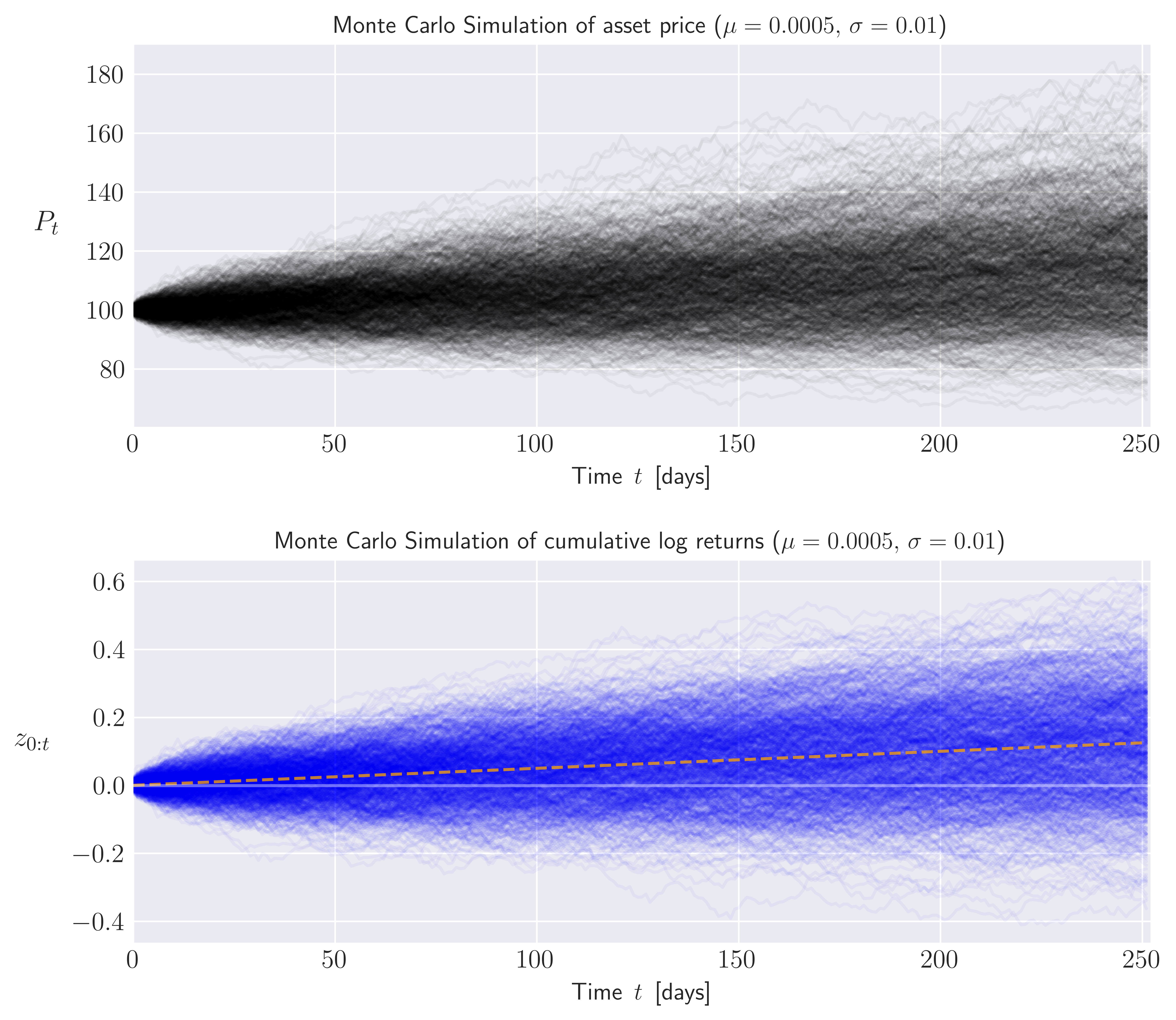Figure 1. One thousand Monte Carlo simulations of the asset price (top) and cumulative log returns (bottom) assuming the asset price follows a Geometric Brownian Motion with daily mean return $\mu = 0.0005$, volatility $\sigma = 0.01$ and initial price of $P_0 = 100$ (USD). The orange dashed line on the bottom panel shows the time evolution of the deterministic drift component.

using the code below:

import matplotlib.pyplot as plt
import matplotlib as mpl

mpl.rcParams['text.usetex'] = True

#For inline plotting 
%matplotlib inline                 
%config InlineBackend.figure_format = 'svg'

plt.style.use("seaborn-v0_8-dark")

fig, axes = plt.subplots(2,1,figsize = (9,8))

axes[0].plot(prices, alpha = 0.04, c = 'black')
axes[1].plot(log_returns, alpha = 0.04, c = 'blue')
axes[1].plot(drifts, alpha = 0.75, c = 'orange', ls = 'dashed')
axes[1].axhline(0, color = 'white', alpha = 0.4)

axes[0].set_ylabel(r'$P_t$', rotation = 0, fontsize = 14, labelpad = 20)
axes[1].set_ylabel(r'$z_{0:t}$', rotation = 0, fontsize = 14, labelpad = 20)

axes[0].set_title(r'Monte Carlo Simulation of asset price ($\mu = 0.0005,\, \sigma = 0.01$)', rotation = 0, fontsize = 12)
axes[1].set_title(r'Monte Carlo Simulation of cumulative log returns ($\mu = 0.0005,\, \sigma = 0.01$)', rotation = 0, fontsize = 12)

for i in range(2):
    
    axes[i].set_xlabel(r'Time $\,t$\, [days]', rotation = 0, fontsize = 12)
    axes[i].set_xlim(0,252)
    axes[i].grid()

plt.subplots_adjust(hspace = 0.35)

To verify our results we can compare the distribution of log-returns obtained at the end point $T = 252$ of our simulations with the theoretical quantities. For example given the expression \eqref{log_ret}, we expect the log-returns to be distributed normally $z_t \sim \mathcal{N}(\mu,\sigma)$ with

\[\begin{equation}\label{dist1} \mathbb{E}[z_t] = \mu, \quad\quad \mathbb{V}[z_t] = \sigma^2 \end{equation}\]

Similarly, given as a sum of independent random variables $z_t$, we expect the cumulative log-returns (see eqs. \eqref{cum_log_ret_d} and \eqref{cum_log_ret}) to exhibit normal distribution $z_{0:T} \sim \mathcal{N}(\mu T, \sigma \sqrt{T})$. This is simply because $z_t$’s that make up $z_{0:T}$ are independent such that their variance of the latter is given by

\[\begin{align} \nonumber \mathbb{E}[z_{0:T}] &= \mathbb{E}\left[\sum_{t = 1}^{T} z_t\right] = \sum_{t = 1}^{T} \mathbb{E}[z_t] = \mu T, \\ \label{dist2}\mathbb{V}[z_{0:T}] &= \mathbb{V}\left[\sum_{t = 1}^{T} z_t\right] = \sum_{t = 1}^{T} \mathbb{V}[z_t] = \sigma^2 T. \end{align}\]

To cross check these expectations, I ran one hundred thousand mc_sims = 100000 simulations using the code block above and compare the resulting distributions with the theoretical normal distributions (see eqs. \eqref{dist1} and \eqref{dist2}), as shown in Figure 2.

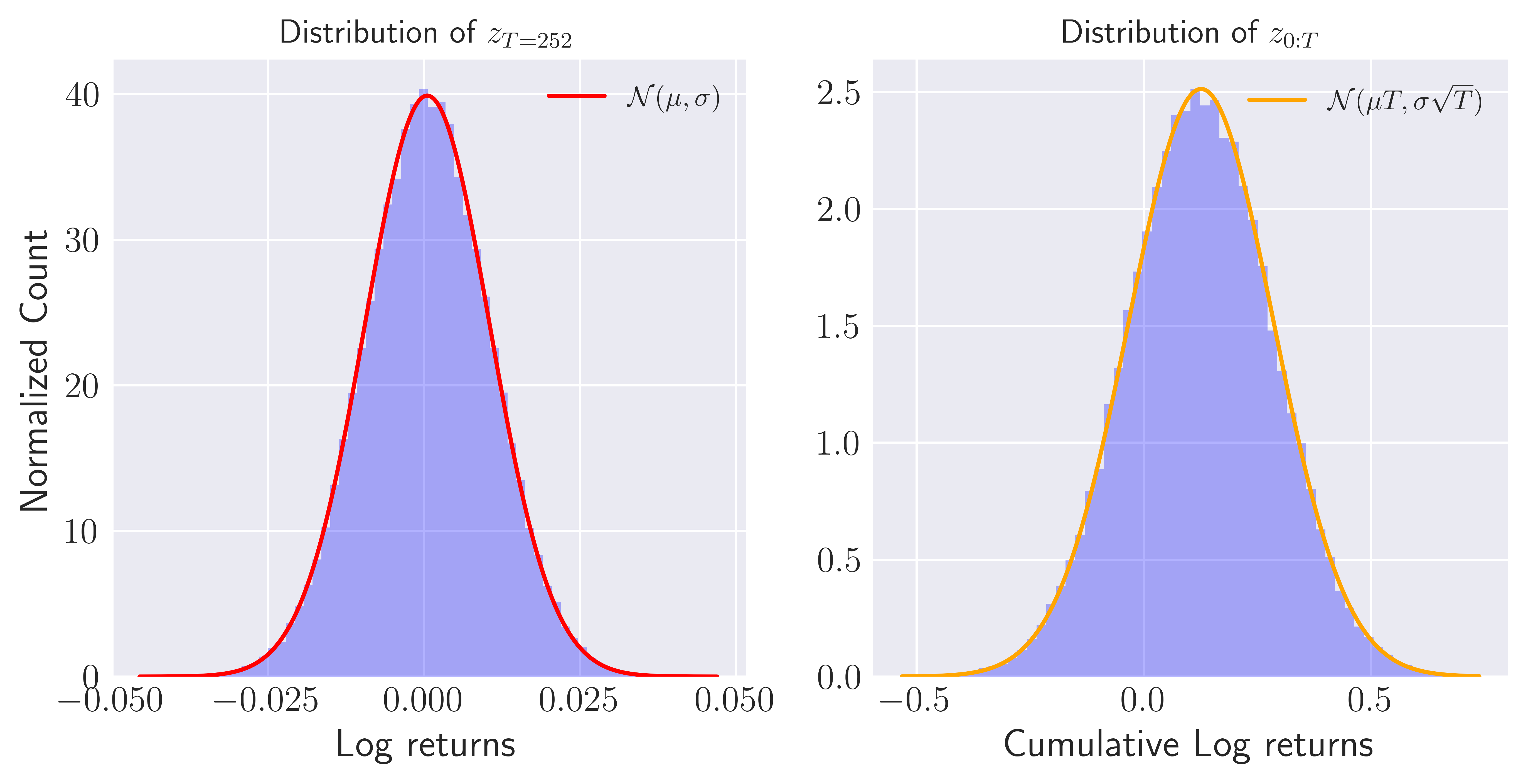Figure 1. Histogram of distributions for log-returns evaluated at the terminal point of simulations (left) and cumulative log-returns (right). Distributions are obtained via mc_sims = 100000 simulations.

The overlap between the theoretical normal distributions with the histograms inform us that our simulations work as expected!. Finally, lets quantitatively compare the expected value of both distributions:

print(f'Expected log-returns at the terminal point, theory vs simulations {mu, daily_log_returns[-1,:].mean()}\n')
print(f'Expected cumulative log-returns, theory vs simulations {mu * T, cum_log_rets.mean()}')

Output:

Expected log-returns at the terminal point, theory vs simulations: (0.0005, 0.000502319592675589)

Expected cumulative log-returns, theory vs simulations: (0.126, 0.12585937531220395)

Notice that theoretical quantities are very close to the results obtained through the Monte Carlo simulations.

I would like to close this post by stressing the similarities between two distributions shown in Figure 2. Both $z_t$ and $z_{0:T}$ are stochastic variables that has its basis on the theory of random walks but they describe the same stochastic process in two different scales: while the former describe the individual steps, the latter corresponds to the end-to-end displacement or price movement. Once we remember the self-similarity property of a random walk, we can make sense of the results shown in Figure 2. as the self-similarity property tells us that a random walk show similar statistical properties, independent of the detail at which it is observed!