Bootstrapping your yield curve

Introduction

---

In this post, we’ll walk through the process of constructing a zero-coupon yield curve using a combination of historical LIBOR and par swap rates. While this approach has been foundational in fixed income finance for decades, it’s worth noting right from the start: LIBOR is no longer used in practice: see e.g. an earlier post.

Since 2021, global financial markets have transitioned away from LIBOR due to its manipulation scandals and declining market activity. Today, rates like SOFR (Secured Overnight Financing Rate) in the U.S. or CORRA in Canada have taken its place. That said, many models, textbooks, and historical datasets still rely on LIBOR and swaps for teaching and legacy applications — making this exercise not only educational, but also a valuable step in understanding the evolution of interest rate modeling.

Why Construct a Yield Curve?

The yield curve — especially the zero-coupon (or spot rate) curve — is the backbone of modern finance. It’s used to:

• Price and hedge fixed-income securities and derivatives
• Extract forward rates and discount factors
• Measure market expectations about future interest rates and economic conditions
• Assess risk and performance in bond portfolios
• Support risk management models in banks and investment firms

In short, constructing a yield curve helps translate the noisy, real-world prices of instruments like short-term loans (LIBOR) and long-term swaps into a clean, arbitrage-free set of rates we can use to price everything else.

What We’ll Do

In this post, we’ll:

1. Use a dataset of historical USD LIBOR and swap rates (circa early 2000s).
2. Build the zero curve step by step using simple bootstrapping techniques.
3. Visualize and interpret the shape of the curve — including why it might rise, flatten, or even dip at the long end.

Fetching and Preparing the Data

---

I originally planned to use the Federal Reserve’s public Python API to fetch historical LIBOR rates for the 1M, 3M, 6M, and 12M tenors, along with par swap rates for longer-maturity swap agreements. However, as with their real-world retirement, LIBOR rates are no longer available through the Fed’s data portal. This reflects the same concerns that led to LIBOR being phased out in practice — mainly the manipulation scandals and the lack of actual underlying transactions in the post-crisis money markets.

Since I still wanted to replicate a historical yield curve construction process (as it was commonly done before the transition to SOFR), I turned to alternative sources. A quick search led me to this page, which offers monthly (obtained via the averages of daily rates) USD LIBOR data going back prior to the 2008 crisis.

For swap rates, I was able to retrieve historical data from the Federal Reserve’s H.15 release, which still includes par swap rates for longer tenors (e.g., 2Y, 3Y, 5Y, 7Y, 10Y, 30Y). These will serve as our inputs for constructing the longer end of the zero-coupon yield curve.

Importing the standard dependencies, we ping the fred API to get the par swap rates:

from fredapi import Fred

api_key = 'your_api_key'

fred = Fred(api_key=api_key)  # Replace with your actual key


start_date = '2004-01-01'
end_date = '2007-01-01'

swap_codes = {
    '2Y': 'DSWP2',
    '3Y': 'DSWP3',
    '5Y': 'DSWP5',
    '7Y': 'DSWP7',
    '10Y': 'DSWP10',
    '30Y': 'DSWP30'
}

# Helper to download series
def download_series(fred, codes):
    return {
        tenor: fred.get_series(code, observation_start=start_date,
                               observation_end=end_date).dropna()
                               for tenor, code in codes.items()
    }

#swap data
swap_data = download_series(fred, swap_codes)
df_swap = pd.DataFrame(swap_data)

df_swap.head()

Output:

	2Y	3Y	5Y	7Y	10Y	30Y
2004-01-02	2.27	2.89	3.79	4.29	4.78	5.49
2004-01-05	2.28	2.91	3.79	4.30	4.79	5.51
2004-01-06	2.19	2.80	3.67	4.19	4.68	5.41
2004-01-07	2.15	2.76	3.62	4.14	4.64	5.40
2004-01-08	2.17	2.77	3.62	4.14	4.63	5.39

We get the LIBOR rates following the link above. These are monthly average rates, so we should re-sample the swap rate time-series to monthly frequency. We finally join the two data frames using the same date ranges:

#read by skipping the metadata rows
libor_rates = pd.read_csv('data/hist_libor_rates_1986-2016.csv', skiprows=16)
libor_rates.columns = ['Date', '1M', '3M', '6M', '12M']


# Convert date column to datetime format
libor_rates['Date'] = pd.to_datetime(libor_rates['Date'])

# Set date as index 
libor_rates.set_index('Date', inplace=True)


s_ts = df_swap.index[0]
e_ts = df_swap.index[-1]

libor_rates = libor_rates[(libor_rates.index >= s_ts)
                           & (libor_rates.index <= e_ts)]

# resample swaps to monthly frequency by taking the average of daily rates

swap_df_monthly = df_swap.resample('MS').mean() 

yield_curve_df = libor_rates.join(swap_df_monthly, how='inner')

yield_curve_df.head()

Output:

	1M	3M	6M	12M	2Y	3Y	5Y	7Y	10Y	30Y
2004-02-01	1.10	1.12	1.17	1.37	2.053158	2.634211	3.451579	3.971053	4.465263	5.250000
2004-03-01	1.09	1.11	1.16	1.35	1.867391	2.383043	3.157826	3.684348	4.194783	5.045652
2004-04-01	1.10	1.18	1.38	1.83	2.377143	2.969524	3.784762	4.284286	4.753333	5.467143
2004-05-01	1.11	1.32	1.58	2.06	2.898500	3.526000	4.326500	4.792500	5.209000	5.797000
2004-06-01	1.37	1.61	1.94	2.46	3.168571	3.709048	4.401429	4.827143	5.220476	5.801429

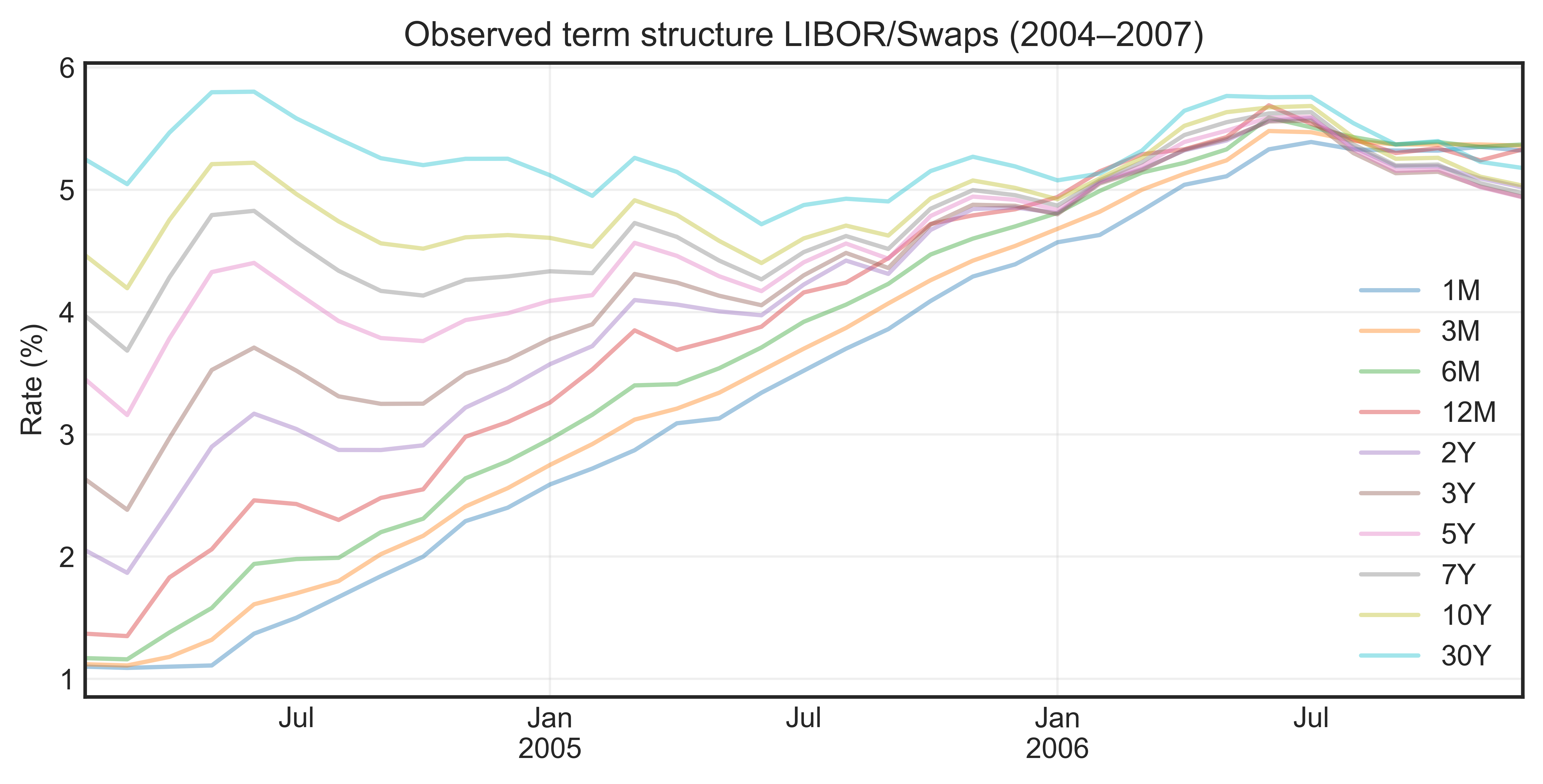Figure 1. Market rates between 2004-2007.

Between 2004 and 2007, long-term swap rates such as the 10-year and 30-year remained relatively stable despite the Federal Reserve steadily raising short-term interest rates. This stability can be attributed to well-anchored long-term (low) inflation expectations, which limited upward pressure on long-term yields. Additionally, markets likely anticipated that the rate hikes would be temporary, with short-term rates eventually declining — keeping the average expected future rates, and thus long-term swap rates, largely unchanged.

Notice that what we have plotted is just market quotes at specific maturities (what’s sometimes called the market curve or observed term structure). On the other hand, a yield curve is a snapshot of interest rates for different maturities at one point in time. We thus want to produce a continuous spot rate curve (zero-coupon yield curve) for each date so that

• Every maturity has a corresponding zero rate.

• We can price any cash flow at any future time from it.

We’ll build the curve one maturity at a time, turning observed market rates into discount factors $P(t_0 = 0, t)$ then into zero rates $z$ via:

\[P(0,t) = \mathrm{e}^{-z(t) t},\quad\quad \rightarrow \quad\quad z(t) = - \frac{\ln P(0,t)}{t}.\]

For short maturities, we do not have to do much as LIBOR is a simple, single-period deposit rate with no intermediate coupon payments. That means the quoted rate for, say, 3M LIBOR is the market’s agreed zero rate for lending/borrowing for exactly 3 months starting now. We do not need to bootstrap — each quote (for a given day) already corresponds to a single discount factor. Thus, using simple compounding, the discount factor (e.g. the value of 1 USD from $T$ years today $t = 0$) is given by

\[P(0,T) = \frac{1}{1 + r_{\rm LIBOR}(T) \, T}\]

where $T$ is in years and $r_{\rm LIBOR}(T)$ is the observed LIBOR rates for a given maturity.

Extending the Yield Curve with Swap Rates

---

To extend the yield curve to longer maturities, we will utilize the observed swap rates. Swap rates provide market-implied information about interest rates over horizons that exceed the maturities of directly traded instruments such as LIBOR deposits or short-term Treasury bills. Before using them for bootstrapping, let us review what an interest rate swap is and how its pricing works.

Plain-vanilla interest rate swap:

• Two parties agree to exchange interest payments on a notional amount $N$ over a fixed schedule of dates $t_1,t_2,\dots,t_n$

• One side pays fixed: a constant rate $K$ agreed upon at inception, multiplied by the notional and the accrual factor for each period.

• The other side pays floating: a short-term market rate (e.g., 3M LIBOR) that resets periodically.

Typical structure;

• Payment frequency: often semiannual for fixed leg, quarterly for floating leg (but market conventions vary by currency).

• Notional exchange: usually not exchanged in vanilla swaps; it’s only used to calculate payments.

At the inception of the contract $t_0$, no money changes hand (swap has zero value). This is achieved when the Present Value of the future cash flows at both side of the contract is equal:

\[\textrm{PV}_{\rm fixed}(t_0,K) = \textrm{PV}_{\rm float}(t_0)\]

The fixed rate $K$ that satisfies this equality is called the par swap rate — directly analogous to a par yield for bonds (where the coupon is set so price = par value).

At the fixed leg, the present value of the cash-flows on a notional amount of $N$ is given by

\[\textrm{PV}_{\rm fixed}(t_0,K) = N \cdot K \sum_{i = 1}^{n} \Delta_i\,P(t_0,t_i)\]

where $\Delta_i$ is the accrual period between $t_{i-1}$ and $t_i$.

So we can say that the fixed leg is equivalent to a bond with coupons equal to $N K \Delta_i$ each payment period without a notional return, at the maturity.

On the other hand, the floating leg of a vanilla interest rate swap can be considered to be economically equivalent to a floating rate note (FRN) that:

• Pays interest every period, where each coupon is determined at the start of the period using the prevailing market rate for that maturity (e.g., 6M LIBOR fixing). However, in valuation terms, since future fixings are unknown, we replace them with forward rates implied by the current zero-coupon curve for the relevant accrual period.

• The principal is conceptually “returned” at maturity, even though notionals are not exchanged in the swap.

In other words,

• In real life → The coupon payments are set literally by the published LIBOR, fixed at the start of each accrual period.

• In valuation models → We use forward rates derived from today’s curve because they’re the arbitrage-free expected rates under the risk-neutral measure:

\[N \cdot f_i\cdot \Delta_i,\]

where $f_i = f(t_0, \Delta_i)$ is the forward rate for the period $\Delta_i$. Therefore, the present value of the cash-flows on the floating leg is given by

\[\textrm{PV}_{\rm float}(t_0) = N \cdot \sum_{i = 1}^{n} f_i\,\Delta_i\,P(t_0, t_i).\]

This expression can be simplified using no-arbitrage condition by re-writing the forward rate for the time period $\Delta_i$ in terms of the discount factors:

Noting $t_0 < t_{i-1} < t_{i}$ and the corresponding zero-rates $r_i$ and $r_{i-1}$

\[(1 + r_i (t_i - t_0)) = (1 + r_{i-1} (t_{i-1} - t_0)) (1 + f_i \Delta_i)\]

which simply tells us that investing at a longer time at fixed rate should be equivalent to investing on shorter periods that sums to the original. Notice that we can re-write the expression above as

\[f_i \Delta_i = \frac{P(t_0, t_{i-1})}{P(t_0, t_{i})} - 1.\]

Plugging it in the present value expression of the floating leg thus gives

\[\textrm{PV}_{\rm float}(t_0) = N \cdot \sum_{i = 1}^{n} [P(t_0, t_{i-1}) - P(t_0, t_{i})] = N [1 - P(t_0,t_n)]\]

Equating the present values of the both legs gives us the par swap rate as

\[K = \frac{1 - P(t_0,t_n)}{\sum_{i = 1}^{n} \Delta_i\,P(t_0,t_i)}\]

This is the core bootstrapping equation we will utilize to extend the yield curve using observed swap rates. The main logic is as follows:

• We already know the short end discount factors $P(0,t_i)$ from LIBOR deposits (e.g., 1M, 3M, 6M, 12M).
• For a swap with maturity $t_n$, we thus the first $n-1$ discount factors from LIBOR and shorter swaps, using which we build the zero curve for longer maturities.

For this purpose, we can re-arrange the expression above and solve for the unknown $P(t_0,t_n)$:

\[\begin{equation} P(t_0,t_n) = \frac{1 - K \sum_{i = 1}^{n-1} \Delta_i\,P(t_0,t_i)}{1 + K \Delta_n} \end{equation}\]

In summary:

1. Start with LIBOR to get $P(0, t_i)$ for the first year.

2. Take the first swap maturity (e.g., 2Y):

   • Plug in the corresponding $K$, the par swap rate from market data.
   • Plug in known $P(0, t_i)$ for all earlier maturities.
   • Solve for the unknown $P(0, t_n)$ at 2Y using the swap pricing formula in eq. (1)

3. Move to the next swap maturity (e.g., 3Y), and repeat:

   • Use the new par rate $K$.
   • Use previously solved $P(0, t_i)$ values.
   • Solve for the new $P(0, t_n)$.

4. Continue this process until you have all discount factors $P(0, t)$ up to the longest maturity (e.g., 30Y).

5. Convert discount factors into continuously compounded zero rates using:

   \[z(t) = -\frac{1}{t} \ln P(0, t)\]

To this end, we first extract LIBOR and par swap rate columns and their maturities in years:

import re

def parse_tenor(tenor_str):
    """Convert tenor strings like '1M', '6M', '2Y' to year fractions."""
    match = re.match(r'(\d+)([MY])', tenor_str)
    if not match:
        raise ValueError(f"Unrecognized tenor format: {tenor_str}")
    num, unit = int(match.group(1)), match.group(2)
    return num / 12 if unit == 'M' else num * 1.0

def infer_columns_and_tenors(df):
    """Automatically determine LIBOR vs. swap columns and tenor values."""
    libor_cols = [col for col in df.columns if col.endswith('M')]
    swap_cols = [col for col in df.columns if col.endswith('Y')]
    
    tenor_to_years = {col: parse_tenor(col) for col in libor_cols + swap_cols}
    return libor_cols, swap_cols, tenor_to_years

libor_columns, swap_columns, tenor_to_years = infer_columns_and_tenors(yield_curve_df)

and then bootstrap assuming the fixed leg/floating legs of the swap agreements both make quarterly payments:

fixed_leg_accrual = 0.25  # in years (change to 0.5 for semi-annual)

def bootstrap_zero_curve(row):
    
    discount_factors = {}

    # Step 1: Calculate discount factors from LIBOR simple compounding
    for col in libor_columns:
        t = tenor_to_years[col]
        rate = row[col] / 100  # convert to decimal
        # Simple compounding discount factor
        discount_factors[t] = 1 / (1 + rate * t)

    # Step 2: Bootstrap discount factors from swap par rates
    for col in swap_columns:
        T = tenor_to_years[col]
        K = row[col] / 100  # par swap rate as decimal

        # Sum the PV of fixed coupons before maturity T
        known_pvs = 0.0
        for t in sorted(discount_factors):
            if t < T:
                known_pvs += K * t * discount_factors[t]

        # Calculate discount factor at maturity T using swap formula
        DF_T = (1 - known_pvs) / (1 + K * fixed_leg_accrual)
        discount_factors[T] = DF_T

    # Step 3: Convert discount factors to continuously compounded zero rates
    zero_rates = {}
    for t, DF in discount_factors.items():
        if DF <= 0:
            # Avoid math errors with log of zero or negative
            zero_rate = np.nan
        else:
            zero_rate = -np.log(DF) / t
        # Label: months for <1 year, else years
        label = f"{int(t*12)}M" if t < 1 else f"{int(t)}Y"
        zero_rates[label] = zero_rate

    return pd.Series(zero_rates)

# Apply to entire DataFrame
zero_curve_df = yield_curve_df.apply(bootstrap_zero_curve, axis = 1)

zero_curve_df.head()

Output:

	1M	3M	6M	1Y	2Y	3Y	5Y	7Y	10Y	30Y
2004-02-01	0.010995	0.011184	0.011666	0.013607	0.021560	0.036680	0.051811	0.076339	0.103865	0.094650
2004-03-01	0.010895	0.011085	0.011566	0.013410	0.019582	0.033093	0.047171	0.070380	0.096728	0.090331
2004-04-01	0.010995	0.011783	0.013753	0.018135	0.024966	0.041415	0.056990	0.082760	0.111331	0.098661
2004-05-01	0.011095	0.013178	0.015738	0.020391	0.030529	0.049386	0.065523	0.093344	0.123153	0.102432
2004-06-01	0.013692	0.016068	0.019307	0.024302	0.033365	0.051913	0.066429	0.093612	0.122654	0.101177

We finally plot the bootstrapped zero curve for three different dates:

# List of dates you want to plot (make sure they exist in zero_curve_df)
dates_to_plot = ['2004-02-01', '2005-02-01', '2006-02-01']

def to_years(tenor):
    num = int(tenor[:-1])
    unit = tenor[-1]
    return num / 12 if unit == 'M' else num

maturities = [to_years(t) for t in zero_curve_df.columns]

plt.figure(figsize=(9, 4))

for date in dates_to_plot:
    zero_rates = zero_curve_df.loc[date]
    plt.plot(maturities, zero_rates.values, alpha = 0.4, marker='o', label=date)

plt.title('Zero Yield Curves on Selected Dates')
plt.xlabel('Maturity [years]')
plt.ylabel('Zero Rate')
plt.legend()
plt.grid(alpha=0.3)

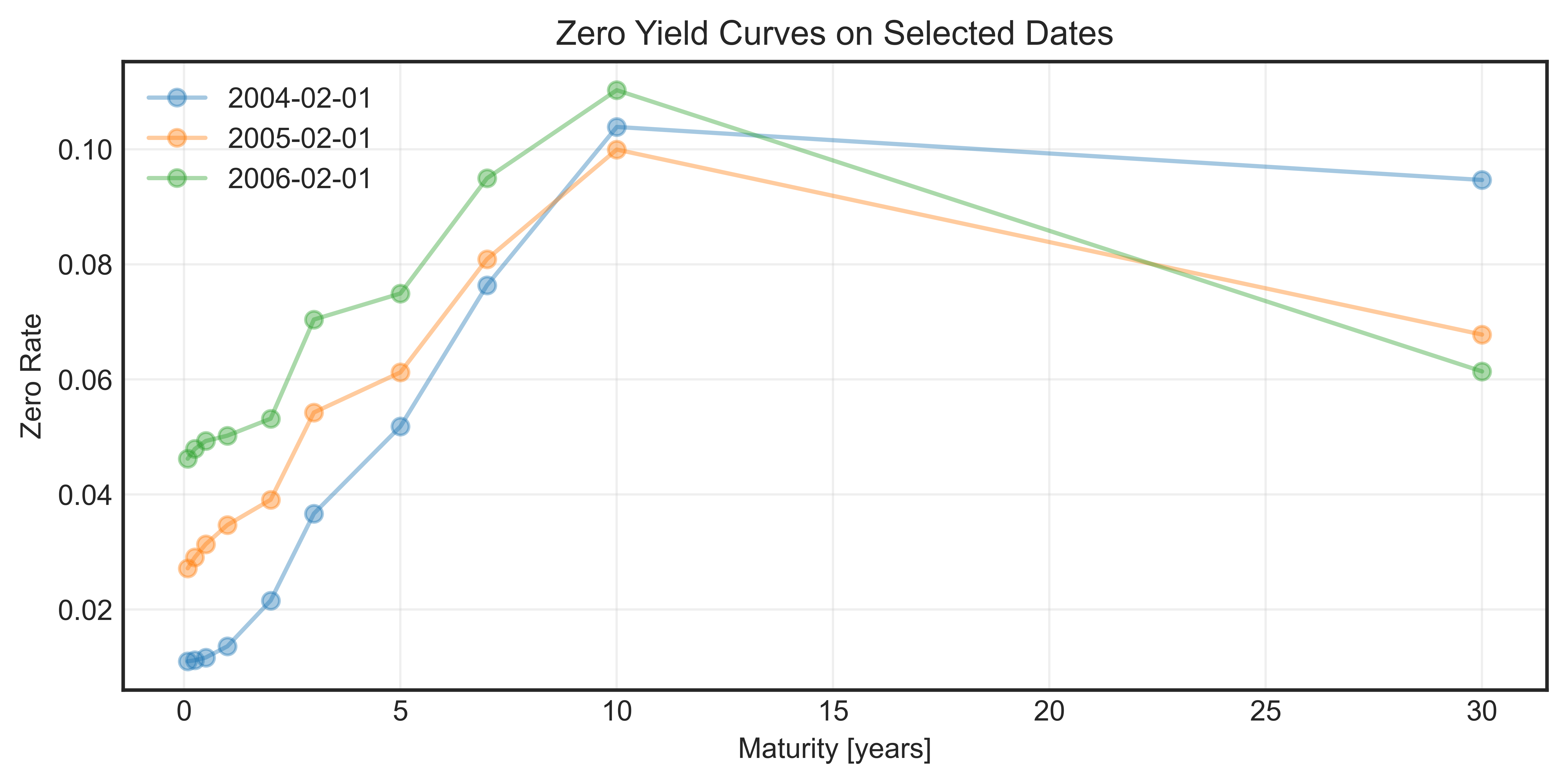Figure 2. Yield curve for three different dates.

The resulting shape of the zero yield curve is sensible from the perspective of market expectations. In particular:

1. The rising rates for the 0-10 years segment is because

   • Inflationary expectations: Investors expect future inflation to be higher than current inflation, so the lenders demand higher yields to compensate for the loss of purchasing power.
   • Term premium: Longer term loans carry more uncertainty and risk due to unexpected inflation, possibility of counterparty defaults and illiquidity. To take on such risks, investors want extra return — this is the term premium, which increases with maturity.

2. Beyond 10 years, the flattening or slight inversion of rates arise because

   • Stabilization of inflation and growth expectations: investors do not expect radically higher rates in the long run as compared to 10 years because central banks (like the Fed or BoC) often aim to anchor inflation expectations in the long term.

   • Demand for long-Term bonds: Institutions like pension funds and insurers need long-dated liabilities. They buy lots of long-term bonds, which increases demand and pushes prices up, which means yields down.