Black-Scholes option pricing
I discuss the standard shortcut of deriving Black Scholes PDE for option pricing with a critical look at its assumptions.
In a previous post, I focused on a simplified single step binomial tree for the evaluation of European vanilla options. By taking advantage of the simple structure of the tree, we tried to gain more insight into the two main ideas that are fundamental in the development of Black-Scholes option pricing theory, namely no-arbitrage and risk-neutrality. In this post, we will follow the same principles to derive the standard continuous model with an aim to have a critical look at its assumptions.
Black-Scholes partial differential equation
Once again, it is useful to put ourselves in the shoes of an option dealer. As a (call) option seller, we know that there is always the possibility that the underlying stock price might end up deep in the money, $S_T \gg K$ at the time of maturity $T$ of the contract. If we do not hold the underlying asset $S$ during the contract, we need to buy it from the market by paying $S_T$ and deliver our obligation to sell it to the counterparty at a fixed price $K$ (strike price). In this world state, our losses $S_T - K \gg 0$ could be well above the premium we charge at the inception of the contract. Of course, we could as well try to incorporate such risks when we price the call option. However, this would require speculating on the future behavior of the underlying stock. However, a market makers job is not to speculate in way to influence the pricing by incorporating such risks.
Therefore, to remove the risks associated with the underlying behavior we require a hedging strategy independent of the future behavior of the stock. In other words, we must make a decision on the basis of the information available today. Without a foreknowledge, we can therefore buy a certain amount of the underlying and continuously adjust this amount (by trading) during the lifetime of the option contract to insure ourselves. Mathematically, we construct a delta hedged portfolio:
\[\begin{equation} V = \Delta S(t) - C(S,t), \end{equation}\]where $\Delta$ is the (instantaneous) amount of stock we hold to hedge the risk associated with our short position in the option. Here, we would like to think that the change in value of our portfolio come from the change in value of the assets $S$ and $C$ we hold (e.g. we are considering a self-financing portfolio), so that we have
\[\begin{equation}\label{dV} \mathrm{d}V = \Delta \mathrm{d} S - \mathrm{d}C. \end{equation}\]Assuming the underlying follows a geometric Brownian motion (GBM) with constant drift $\mu$ and volatility $\sigma$:
\[\begin{equation}\label{gbm} \mathrm{d}S = \mu S \, \mathrm{d}t + \sigma S\, \mathrm{d}W, \quad\quad \mathrm{d}W \sim \mathcal{N}(0,\mathrm{d}t), \end{equation}\]we first explore the change in our portfolio \eqref{dV} in terms of the change in the value of the option, using Ito’s lemma we have
\[\begin{align} \nonumber \mathrm{d}V &= \Delta \mathrm{d}S - \left(\frac{\partial C}{\partial t} \mathrm{d}t + \frac{\partial C}{\partial S} \mathrm{d}S + \frac{1}{2} \frac{\partial^2 C}{\partial S^2} \mathrm{d}S^2 \right),\\ & = \left(\Delta - \frac{\partial C}{\partial S}\right)\mathrm{d}S - \left(\frac{\partial C}{\partial t} \mathrm{d}t + \frac{1}{2} \frac{\partial^2 C}{\partial S^2} \mathrm{d}S^2 \right).\label{dV2} \end{align}\]Recall that our goal with constructing this portfolio was to hedge our risk associated with the movements of the stock prices which follows a GBM. We have two potentially risky terms that can cause an uncertainty in the change of the portfolio value. The first one is $\mathrm{d} S^2$ term. However, by Ito’s lemma, we actually know that this term is deterministic as long as we constrain ourselves with infinitesimal time increments $\mathrm{d}t$, as its variance caused by the Brownian motion is quadratic in the latter:
\[\begin{equation} \mathrm{d}S^2 \to \sigma^2 S^2 \mathrm{d}W^2 \to \sigma^2 S^2 \mathrm{d}t, \quad\quad \textrm{for} \quad \mathbb{E}[\mathrm{d}W^2] = \mathrm{d}t, \quad \mathbb{V}[\mathrm{d}W^2] = \mathcal{O}(\mathrm{d}t^2) \simeq 0. \end{equation}\]This leaves us with the first term in \eqref{dV2} proportional to $\mathrm{d}S$. To remove all the uncertainty, the change in our portfolio value should worth the same in all states of the world that may arise due to the stochastic Brownian motion of the underlying. We can simply achieve this by simply setting the first term in \eqref{dV2} to zero:
\(\begin{equation}\label{dh} \Delta = \frac{\partial C}{\partial S}. \end{equation}\) This implies that we are adopting a trading strategy where we hold $\Delta$ amount of the asset according to the sensitivity of the option to the underlying. In this way, we remove the sensitivity of our portfolio to the underlying, and we totally hedged our risk. Since the portfolio is risk-free tomorrow (e.g. at time $t + \mathrm{d}t$), it should evolve under the laws of the risk-free rate, between time $t$ and $t + \mathrm{d} t$:
\[\begin{equation}\label{dVrn} \mathrm{d} V = r\, V \mathrm{d}t = r \left(\frac{\partial C}{\partial S}\,S - C\right) \mathrm{d} t. \end{equation}\]Equating \eqref{dVrn} with \eqref{dV2} and using the Delta hedging \eqref{dh}, we derive dynamics of a call option as a partial differential equation (PDE)
\[\begin{equation}\label{BS} \frac{\partial C}{\partial t} + r\,S\, \frac{\partial C}{\partial S} + \frac{\sigma^2\,S^2}{2} \frac{\partial^2 C}{\partial S^2} = r\,C. \end{equation}\]This is the famous Black-Scholes partial differential equation (PDE) for a call option.
Notice that $\Delta$ hedging not only removed potential stochastic terms that may appear in \eqref{BS}, but also rendered it independent of the drift of the underlying asset, $\mu$. In the context of GBM \eqref{gbm}, $\mu$ can be considered as the premium investors demand due to riskiness of the stock. Our hedging argument simply removed this dependence in the Black-Scholes PDE. In fact, as it should be clear from eq. \eqref{dVrn}, in the Black-Scholes world, our portfolio and hence the assets ($S,C$) that make up the portfolio evolve with the risk-free rate. In other words, we say that the pricing implied by the solution to the Black-Scholes PDE is the risk-neutral pricing. In this world, investors do not demand an additional reward ($\mu$) to compensate the riskiness of the asset and so that all the assets evolve as if they are riskless bonds! These arguments are also consistent with the no-arbitrage principle: Since we hedged the option, our portfolio value agrees with the amount of riskless bonds in every state of the world at time $t + \delta t$, e.g. for an investment of $V(t)$ amount to a money market account that has a short rate of interest $r$. Our portfolio must therefore have a value of $V(t)$ at time $t < t + \delta t$ because otherwise arbitrage opportunities appear. This is essentially what is implied by eq. \eqref{dVrn}:
\[\begin{equation} V(t+\delta t) = V(t)\, \mathrm{e}^{r\delta t}. \end{equation}\]Solving the Black-Scholes equation
As a second order partial differential equation, the Black-Scholes equation \eqref{BS} has many solutions. To determine a unique solution, we require an additional constraint. In fact, we certainly know the value of our call option at the expiry $t = T$:
\[\begin{equation}\label{bc} C(S,T) = (S(T) - K)_{+} = \textrm{max}(S(T)- K, 0), \end{equation}\]as the option would be exercised if and only if $S(T) > K$. It is important the emphasize that, only at this point the fact that we are dealing with a call option comes into picture. We could as well repeat the same analysis above for any European contingent claim (derivative), whose pay-off is determined as a function of the underlying price $S$ at the time of expiry $T$: $C(S,T) = f(S)$.
We are now in a position to determine a unique solution to \eqref{BS}. All we need to do is to message it a bit in order to write it in terms of a well known equation. In fact, \eqref{BS} is just the heat equation in disguise. For this purpose, we perform the following transformations in order:
By taking advantage of the form of the partial derivatives w.r.t $S$ in \eqref{BS}, we let $S = \mathrm{e}^Z \to \ln S = Z$.
Since we are interested in the price of the option w.r.t the time to maturity, we define a new time variable $\tau = T - t$.
Next, we eliminate the term proportional to $r C$ in the right-hand side of \eqref{BS} by defining a new variable via $D = \mathrm{e}^{r\tau}\, C$. This makes sense since we are interested in the value of the possible cash-flow in the future: $C = \mathrm{e}^{-r\tau}\, D$.
The final transformation give rise to a linear term: $(r - \sigma^2/2) \partial D / \partial Z$ which we can eliminate by noticing that the price of the underlying that follows a GBM \eqref{gbm} has a solution of the form (in a distributional sense): $Z = Z(0) + (r - \sigma^2/2)t + \dots$ where dots denote the term proportional to Wiener process. We can therefore shift the “spatial” coordinate we defined earlier by taking into account the mean of the $Z$, e.g. by defining $y = Z + (r - \sigma^2/2)\tau$.
Following these steps lead us to the one dimensional heat equation:
\[\begin{equation}\label{he} \frac{\partial D}{\partial \tau} = \frac{\sigma^2}{2} \frac{\partial^2 D}{\partial y^2}. \end{equation}\]Transforming the boundary condition \eqref{bc} in terms of the new variables we have:
\[\begin{equation}\label{dbc} D(y_T,\tau = 0) = K\textrm{max}(\mathrm{e}^{y_T - \ln K} - 1, 0), \end{equation}\]general solution to \eqref{he} can be derived using Green’s function method which simply generates solutions in terms of the boundary condition at $\tau = 0$ as
\[\begin{equation}\label{she} D(y,\tau) = \int_{-\infty}^{\infty} G_{\sigma}(y-y', \tau)\, D(y', \tau = 0)\, \mathrm{d}y', \end{equation}\]where $G$ is the Green’s function (also referred as the heat kernel) of the operator $\partial/\partial \tau - (\sigma^2 /2)\partial^2 / \partial y^2$:
\[\begin{equation}\label{gf} G_\sigma(z,\tau) = \frac{1}{\sqrt{2\pi \tau} \sigma} \, \mathrm{e^{-z^2/(2\sigma^2 \tau)}}. \end{equation}\]It is easy to see that the above functional form satisfies \eqref{he}, rendering the solution \eqref{she} as the general solution to the heat equation. Plugging \eqref{dbc}, the general solution is thus given by
\[\begin{align} \nonumber D(y,\tau) &= \frac{K}{\sqrt{2\pi \tau} \sigma} \int_{-\infty}^{\infty} \mathrm{e}^{-(y-y')^2 / (2 \sigma^2 \tau)}\, \textrm{max}(\mathrm{e}^{y' - \ln K} - 1, 0)\, \mathrm{d} y', \\ & = \frac{1}{\sqrt{2\pi \tau}\sigma} \int_{\ln K}^{\infty} \mathrm{e}^{-(y-y')^2 / (2 \sigma^2 \tau)}\, \mathrm{e}^{y'} \mathrm{d} y' - \frac{K}{\sqrt{2\pi \tau}\sigma} \int_{\ln K}^{\infty} \mathrm{e}^{-(y-y')^2 / (2 \sigma^2 \tau)}\, \mathrm{d} y'. \label{Dsol} \end{align}\]The integrals above can be written in terms of the cumulative probability $N(\dots)$ of standard normal distribution. In particular, for the second integral we can define a new variable via $\sigma \sqrt{\tau} z = y-y’$, whereas for the first one we need to complete the exponents to square by carefully considering extra terms that can be taken outside the integral. This can be done by noting that the exponent in the first integrand can be re-written as
\[\begin{equation} \frac{[(y-y') + \sigma^2 \tau]^2}{2\sigma^2 \tau} + (y + \frac{\sigma^2 \tau}{2}). \end{equation}\]We can then define a new variable as $ z’ = [(y-y’) + \sigma^2\tau] /\sigma \sqrt{\tau} $ to render the first integral in \eqref{Dsol} in terms of another cumulative probability on standard normal distribution. Described mathematically, these steps are given by
\[\begin{align} \nonumber D(y,\tau) &= \mathrm{e}^{y + \sigma^2\tau/2} \int_{-\infty}^{(y - \ln K)/(\sigma \sqrt{\tau}) + \sigma \sqrt{\tau}} \frac{\mathrm{e}^{-z'^2/2}}{\sqrt{2\pi}}\, \mathrm{d}z' - K \int_{-\infty}^{(y - \ln K)/(\sigma \sqrt{\tau})} \frac{\mathrm{e}^{-z^2/2}}{\sqrt{2\pi}}\, \mathrm{d}z, \\ & = \mathrm{e}^{y + \sigma^2\tau/2} N\left(\frac{y - \ln K}{\sigma \sqrt{\tau}} + \sigma \sqrt{\tau}\right) - K\, N \left(\frac{y - \ln K}{\sigma \sqrt{\tau}}\right). \end{align}\]We are almost done. The final step is just about returning to the original variables noting $C = \mathrm{e}^{-r \tau} D$, $ y = \ln S + (r - \sigma^2/2)\tau$ with $\tau = T - t$, this lead us to the famous Black-Scholes formulas
\[\begin{equation}\label{bsf} C(S,t;K,T,\sigma,r) = S\, N(d_1) - K\,\mathrm{e}^{-r (T - t)}\, N(d_2) \end{equation}\]where
\[\begin{align} \nonumber d_2 &= \frac{\ln(S/K)+ (r-\sigma^2/2)(T - t)}{\sigma \sqrt{T-t}},\\ d_1 &= d_2 + \sigma \sqrt{T-t}. \end{align}\]Using the put-call parity, we can similarly obtain the price of the puts as:
\[\begin{align} \nonumber P(S,t;K,T,\sigma,r) &= C(S,t;K,T,\sigma,r) - F(S,t),\\ \nonumber &= C(S,t;K,T,\sigma,r) - (S - K\, \mathrm{e}^{-r(T-t)}),\\ \nonumber &= -S(1 - N(d_1)) + K \, \mathrm{e}^{-r(T-t)} (1 - N(d_2)),\\ &= -S N(-d_1) + K \, \mathrm{e}^{-r(T-t)} N(-d_2).\label{bsfp} \end{align}\]There are various ways of interpreting the terms that appear in the Black-Scholes formula \eqref{bsf}. Here is one I find interesting. First, notice that delta of the call option is given by the cumulative probability that appear in the first term:
\[\Delta = \frac{\partial C}{\partial S} = N(d_1).\]On the other hand, the underlying evolving under the risk-neutral GBM \eqref{gbm} ($\mu = r$) has the following solution
\[S_T = \mathrm{e}^{\ln S + (r-\sigma^2/2)(T-t) + \sigma \sqrt{T-t}\, N(0,1)}.\]Therefore, the cumulative distribution that appear in the second term in \eqref{bsf} can be interpreted as the probability $\mathbb{Q}$ that the option ends in the money:
\[\begin{align} \nonumber \mathbb{Q}(S_T > K) &= \mathbb{Q}(\mathrm{e}^{\ln S + (r-\sigma^2/2)(T-t) + \sigma \sqrt{T-t}\, Z} > K),\\ \nonumber &= N(Z > -d_2),\\ &= N(d_2), \end{align}\]where we used the fact that $Z \sim N(0,1)$ and that $N(Z>x) = N(Z\leq-x)$ due to symmetry property of the standard normal distribution. Taking into account the $K\,\mathrm{e}^{-r (T-t)}$ factor, we can interpret the second term in \eqref{bsf} as the discounted value of $K$ zero coupon bounds (each pay $1$ at the maturity $T$) contingent on the option is exercised. Together with the equivalency $\Delta = N(d_1)$, these arguments imply that the value of the call option can be said to be determined by the cost of a portfolio that replicates the option’s value at the pay-off $t = T$. This portfolio consist of $\Delta = N(d_1) > 0$ (e.g. long position) amount of stocks minus K zero coupon bonds (or short K zero coupon bonds). This is the replica trick that is sometimes utilized in the literature to derive the option’s value without consorting on the methods we delved into in this post.
Since the Black-Scholes formulas \eqref{bsf} and \eqref{bsfp} are not so illuminating, one might wonder how does the price evolve with respect to volatility $\sigma$, which is arguably one of the most important parameters of the model.
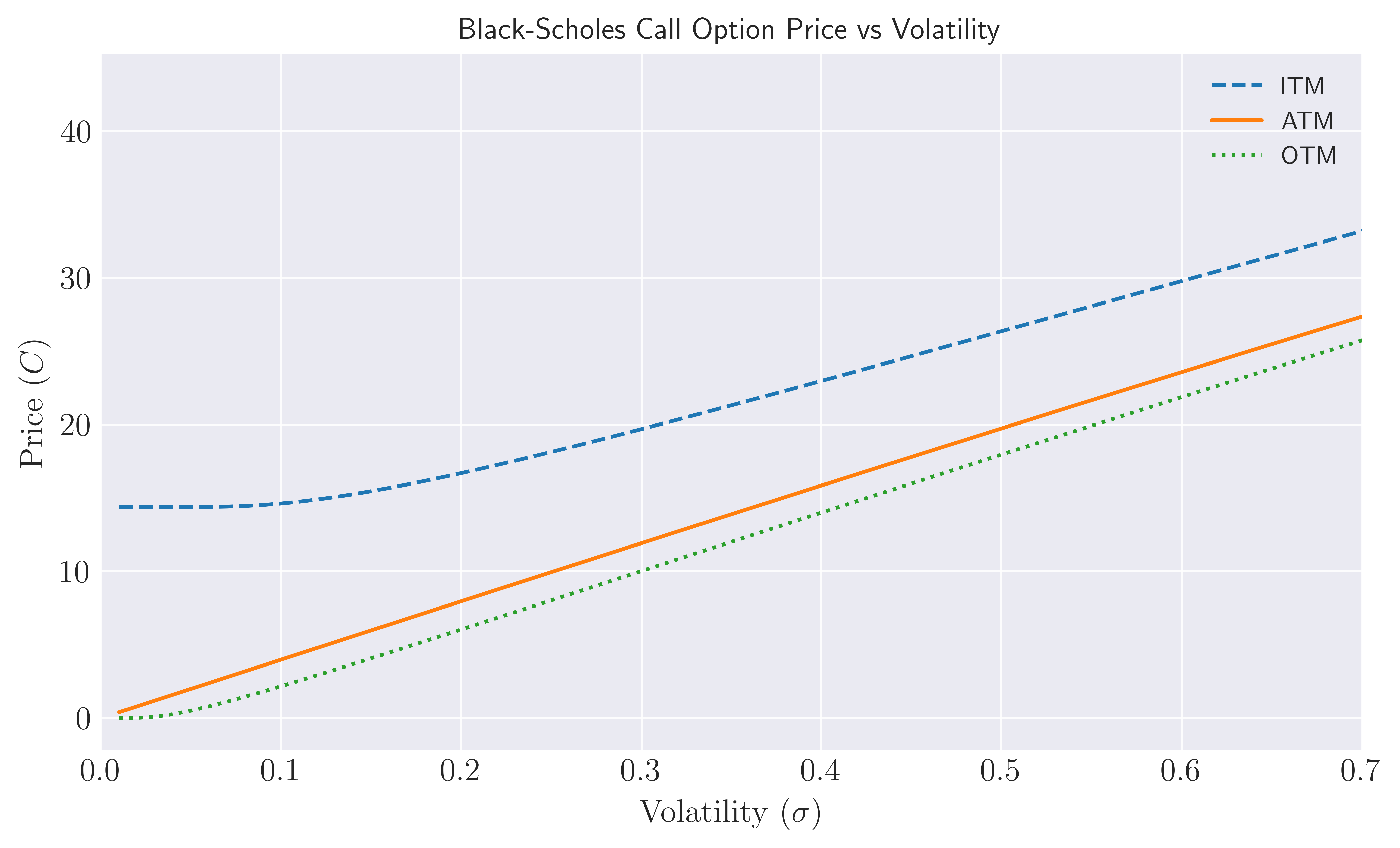 Figure 1. Option price as a function of volatility for a call option that ends at the money (ATM) (orange curve), in the money (ITM) and out of money.The current stock price is set to $S(t = 0) = S_0 = 100$, $r = 0.05$ and $T = 1$ in years.
We show this dependence in Figure 1., for a call option that ends at the money (ATM), $S_T = S_0 \mathrm{e}^{rT} = K \simeq 105$, in the money (ITM) $S_T > K$ ($K = 90$) and out of money (OTM) $S_T < K$ ($K = 110$). Notice that no matter how small the volatility is, price of the call option is always greater than its intrinsic value $S_0 - K$. This is in particularly visible for the in the money option (dashed blue line), where $C(S_0, t = 0) > S_0 - K = 10$. Furthermore, we observe that ATM call options almost exhibit a linear relationship with the price. This relation summarizes nicely the market’s view on volatility: the seller of the option compensate his/her risk by charging in an amount proportional to the volatility of the underlying. In fact, this relationship can be quantified by focusing on the Black-Scholes formula \eqref{bsf} for at the money options $ K= S \mathrm{e}^{r (T-t)}$:
\[\begin{equation} C(S = K e^{-r (T-t)}, t) = S \left[ N\left(\frac{\sigma \sqrt{T-t}}{2}\right) - N\left(-\frac{\sigma \sqrt{T-t}}{2}\right)\right]. \end{equation}\]Focusing on contracts with short time to maturities, or in general for $\sigma \sqrt{T-t} \ll 1$, we can Taylor expand the cumulative probabilities to obtain
\[\begin{equation} \nonumber C(S = K e^{-r (T-t)}, t) \xrightarrow{\sigma \sqrt{T-t} \ll 1} S \left[ N'(0) \sigma \sqrt{T-t} + \mathcal{O}\left((\sigma \sqrt{T-t})^3\right) \right] \simeq S \sigma \sqrt{\frac{T-t}{2\pi}}. \end{equation}\]Convexity vs time decay.
One of the most important characteristic of options as a derivative contract is its asymmetric payoff: while the potential losses are limited, our upside gains are unlimited. Note that this is in contrast with other types of derivatives such as forwards where the pay-off is always linear in the underlying price. In finance, this kind of asymmetric (non-linear) behavior is called “convexity”. This property is already apparent from the pay-off which has a kink at $S_T = K$.
How do we expect the call price to behave before the expiry, i.e. for $T - t > 0$? We might expect it to look like a smoothed version of the final pay-off which would not be surprising recalling that the general solution in \eqref{she} which characterize the smoothing of the final pay-off \eqref{dbc} via the Gaussian Heat Kernel \eqref{gf}. This also makes intuitive sense, because even if the option is out-of-money before the maturity $S \lesssim K$, our long position in the call option is not worthless because it is still possible for the stock price to rise above the strike before expiry. Therefore, we should still be able to sell the contract for more than zero. The closer the stock is to the strike $K$, the more valuable it should be in the views of the market participants. To summarize, the price of the option will change non-linearly with the price of the stock, and we approach to the maturity, the smooth approximation should look more and more like the pay-off function, because the option is losing its optionality for $t \to T$. This struggle between the convexity and the time decay is the fundamental dynamics of the options, which are in fact really nicely captured by the Black-Scholes formula: taking the second derivative of the call option \eqref{bsf} with respect to the stock price (corresponding to the Greek Gamma), we have
\[\begin{equation} \Gamma = \frac{\partial^2 C}{\partial S^2} = \frac{N'(d_1)}{S\sigma \sqrt{T-t}} > 0, \end{equation}\]which is strictly positive (for both puts and calls) noting $N’(z) = \mathrm{e}^{-z^2/2}/\sqrt{2\pi}$. As a consequence, the Black-Scholes price of an option is a convex function of the stock price. We illustrate the convexity and time decaying behavior of the call option prices in Figure 2., where we plot \eqref{bsf} as a function of the spot price $S$ for a given set of time to maturities $T - t$ (assuming $t = 0$).
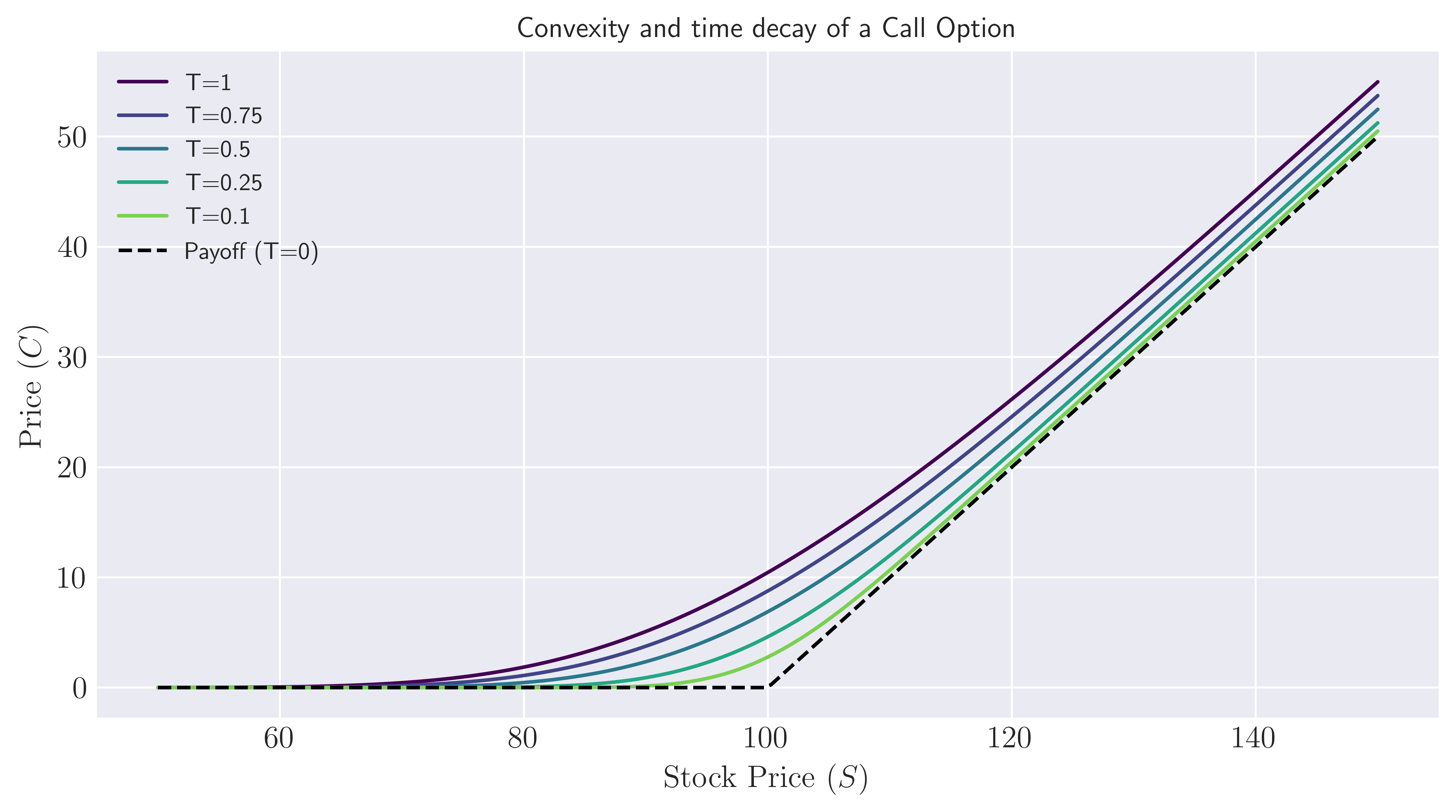 Figure 2. Call option prices at various times before maturity. We assume a call option with strike $K = 100$ on an underling $S$ with 20 percent volatility, $\sigma = 0.2$. Risk-free rate is chosen to be $r = 0.05$.
Shortcomings of the Black-Scholes world
The elegance that the Black-Scholes world provides through simplicity is notwithstanding, the simplifying assumptions it makes are quite far from describing the real world behavior in the option markets. What are the shortcomings of the Black-Scholes pricing model? Notice that the model produces option prices for a given set of parameters/variables. These parameters are the strike $K$, time to maturity $T-t$, current stock price, interest rates $r$ and volatility. The latter has a special position because all the other parameters are either specified in the contract (such as $K$, $T$) or observable in the market ($S$ and $r$). From an option dealer’s perspective the issue is to estimate the volatility during the life of the option. This is typically done by collecting data on the prices of the traded options in the market, which give rise to the concept of implied volatility, e.g. the volatility implied by the price. Empirical data in the option markets show that the implied volatility has a non-trivial dependence on the strike price $K$ even for option’s on the same underlying asset. Typically, the graph of implied volatility with respect to $K$ shows a “smile” type shape that reflects the demand-supply dynamics in the market. Furthermore, the smiles are a consistent feature of the markets: although the precise shape of the implied volatility $\sigma(K)$ will be different due to the nature of the underlying, they are never a flat horizontal line as assumed by the Black-Scholes model! This in practice implies that one needs to at least calibrate the Black-Scholes pricing formulas to be able to match the market prices agree with the model.
Apart from the volatility, the second main assumption that lead us to the pricing formula \eqref{bsf} was the log-normality (or normality) of stock prices (stock returns). In reality, it is known that stock returns exhibit fat tails that are associated with extreme values. This can easily lead to mispricing of European options. This fact shows the model dependence of the Black-Scholes world which relies heavily on the Geometric Brownian motion as the stochastic process that describes the dynamics of the underlying.
In another post, I intend to focus on a less model dependent pricing method called the risk-neutral pricing for which we already showed a glimpse in this post.
References
1. “Derivatives and Internal Models: Modern Risk Management”, Hans-Peter Deutsch and Mark W. Beinker .
2. “The concepts and practice of mathematical finance”, Second Edition, Mark S. Joshi.
Appendix A: Code to reproduce Figure 1
1
2
3
4
5
6
7
8
9
10
11
12
13
14
15
16
17
18
19
20
21
22
23
24
25
26
27
28
29
30
31
32
33
34
35
36
37
38
39
40
41
42
43
44
45
46
47
48
49
import numpy as np
import matplotlib.pyplot as plt
from scipy.stats import norm

import matplotlib as mpl

mpl.rcParams['text.usetex'] = True
plt.rcParams['xtick.labelsize'] = 13
plt.rcParams['ytick.labelsize'] = 13

#For inline plotting
%matplotlib inline
%config InlineBackend.figure_format = 'svg'
plt.style.use("seaborn-v0_8-dark")

# Black-Scholes formula for a European call option
def black_scholes_call(S, K, T, r, sigma):
    d1 = (np.log(S / K) + (r + 0.5 * sigma ** 2) * T) / (sigma * np.sqrt(T))
    d2 = d1 - sigma * np.sqrt(T)
    return S * norm.cdf(d1) - K * np.exp(-r * T) * norm.cdf(d2)

# Parameters
S = 100      # Stock price
T = 1        # Time to maturity (1 year)
r = 0.05     # Risk-free rate (5%)
vols = np.linspace(0.01, 1, 100)  # Range of volatilities

# Define strike prices for ITM, ATM, and OTM options
K_itm = 90    # In-the-money
K_atm = S * np.exp(r * T)   # At-the-money
K_otm = 110   # Out-of-the-money

# Compute call prices for different volatilities
call_prices_itm = [black_scholes_call(S, K_itm, T, r, vol) for vol in vols]
call_prices_atm = [black_scholes_call(S, K_atm, T, r, vol) for vol in vols]
call_prices_otm = [black_scholes_call(S, K_otm, T, r, vol) for vol in vols]

# Plot results
plt.figure(figsize=(9, 5))
plt.plot(vols, call_prices_itm, label="ITM", linestyle="dashed")
plt.plot(vols, call_prices_atm, label="ATM", linestyle="solid")
plt.plot(vols, call_prices_otm, label="OTM", linestyle="dotted")

plt.xlabel(r"$\textrm{Volatility}\,\, (\sigma)$", fontsize = 13)
plt.ylabel(r"$\textrm{Price}\,\, (C)$", fontsize = 13)
plt.title("Black-Scholes Call Option Price vs Volatility")
plt.xlim(0,0.7)
plt.legend()
plt.grid(alpha = 0.9)
Appendix B: Code to reproduce Figure 2
1
2
3
4
5
6
7
8
9
10
11
12
13
14
15
16
17
18
19
20
21
22
23
24
25
26
27
28
29
30
31
32
33
34
35
36
37
import numpy as np
import matplotlib.pyplot as plt
from scipy.stats import norm
import matplotlib.cm as cm

# Black-Scholes formula for European call option
def black_scholes_call(S, K, T, r, sigma):
    if T == 0:
        return max(S - K, 0)  # Payoff at expiry
    d1 = (np.log(S / K) + (r + 0.5 * sigma ** 2) * T) / (sigma * np.sqrt(T))
    d2 = d1 - sigma * np.sqrt(T)
    return S * norm.cdf(d1) - K * np.exp(-r * T) * norm.cdf(d2)

# Parameters
K = 100     # Strike price
r = 0.05    # Risk-free rate
sigma = 0.2 # Volatility

S_values = np.linspace(50, 150, 200)  # Stock price range
T_values = [1, 0.75, 0.5, 0.25, 0.1, 0]

colors = cm.viridis(np.linspace(0, 1, len(T_values)))  # Color map

# 1. Convexity of Call Option Price
plt.figure(figsize=(10, 5))
for i, T in enumerate(T_values):
    call_prices = [black_scholes_call(S, K, T, r, sigma) for S in S_values]
    label = f"T={T}" if T > 0 else "Payoff (T=0)"
    color = colors[i] if T > 0 else "black"
    linestyle = "-" if T > 0 else "--"  # Dashed for final payoff
    plt.plot(S_values, call_prices, label=label, color=color, linestyle=linestyle)

plt.xlabel(r"$\textrm{Stock Price}\,\, (S)$", fontsize = 13)
plt.ylabel(r"$\textrm{Price}\,\,(C)$", fontsize = 13)
plt.title("Convexity and time decay of a Call Option")
plt.legend()
plt.grid()