Single Period Binomial Model

An option is essentially a conditional financial contract that derives its value from an underlying asset. While primitive option-like contracts have been practiced for centuries, the introduction of Black-Scholes model (developed by Fischer Black, Myron Scholes, and later extended by Robert Merton, 1973) revolutionized option pricing by providing a theoretical framework to determine the fair price of European-style options, which led to significant growth (in liquidity) and sophistication in options markets.

The impact of Black-Scholes model in financial markets is notwithstanding, it relies heavily on rather complex mathematical framework of stochastic calculus which I intend to explore in another post. Here, I will focus on a simplified discrete time analog of Black-Scholes Model called the Binomial option pricing model (developed by John Cox, Stephen Ross, Mark Rubinstein, 1979).

In particular, I will consider a second layer of simplification, considering a binomial model with a single time step. This will allow us to grasp the main ideas behind option pricing intuitively and help us explore two key ideas that were fundamental within the realm of Black-Scholes world: namely no-arbitrage principle and risk-neutrality.

Options

---

We begin by defining option contracts for which I will always refer to European style options.

A European option is a financial contract that gives the buyer the right but not the obligation to buy or sell the underling stock/asset at a pre-determined fixed price, called the strike price and on a fixed date, called the exercise date. There are two main types of options exercised in the financial markets: a call option gives the buyer the right to buy the underlying asset, while a put option gives the buyer the right to sell (short) the underlying asset. Furthermore, we can talk about the intrinsic value (parity value) of an option as the value of the option has if exercised immediately, while the premium over parity is the amount by which the market price of an option (or a convertible security) exceeds its parity value (intrinsic value). This premium accounts for the additional value investors are willing to pay beyond the immediate exercise value, reflecting factors like time value of the option.

To warm things up, now consider an option (call or put) with strike price $K$, on an underlying stock with a current price of $S_0$ and imagine that the exercise date is one discrete-time point into the future, i.e. when the stock is valued at $S_1$. What would be the intrinsic (parity) value of the option at the expiry? Assuming holding a call option, a rational investor will certainly exercise the option, if $S_1 > K$ because in doing so would be advantageous as the investor will have the opportunity to buy low and sell the underlying back in the market pocketing $S_1 - K > 0$. If on the other hand $S_1 < K$, the option expires worthless. Therefore, at the expiry the parity value of a call option is worth precisely

\[\begin{equation}\label{Vc} V^{(c)}_1 = \textrm{max}(S_1-K,0) \end{equation}\]

Note that in reality, the total profit she can make by exercising the option would be $S_1 - K$ minus the premium over parity. Similarly, the parity value of a put option at the expiry is

\[\begin{equation}\label{Vp} V^{(p)}_1 = \textrm{max}(K - S_1,0) \end{equation}\]

In this case, if the strike price is greater than the stock, we want to exercise the put option (sell the stock short) for $K$ and then immediately buy it back on the open market for $S_1$, pocketing $K - S_1$ less the premium over parity. If otherwise the stock is worth more than the strike, the put option is worthless.

Notice that both the value of both options have a kink at the strike price. This reflects the non-linearity of the option value with respect to the price of the underlying as it implies a discontinuous change in the value at that point. Furthermore, so far we only mentioned the option value at the expiry, but our main goal is to determine the fair value before its expiry. The time component also introduces another interesting layer to the non-linearity discussion. For example, we can consider a call option prior to the expiry at time $t$ where the stock price $S_t$ is less than the strike $K$. Our call option is not worthless because the underlying has still the potential to jump above the strike before expiry depending on for example factors like stock’s volatility. In fact, the more the stock price $S_t$ closer to the strike, with more amount we should be able to sell our option for. The important point I am trying make here is that any time prior to the expiry, the value of the option will look like a smooth approximation to the piece-wise kinky functions we mentioned above, in a way that depends non-linearly on the stock price and this value curve will look more and more like the piece-wise profile \eqref{Vc} or its mirror function \eqref{Vp} in the case of puts.

One-step binomial tree

---

For the purpose of deriving a fair value for options, we will first focus on the dynamics of the underlying stock within the simplified one step binomial model, as shown in Figure 1.

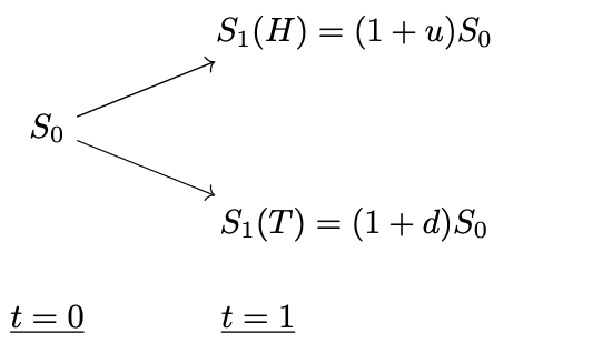Figure 1. One-step binomial model for the underlying dynamics.

At the initial time $t = 0$, we assume that we have a stock whose price is known to be $S_0 > 0$. One step into the future, the stock price $S_1 > 0$ is a random variable that takes up two possible values according to the outcome of a possibly biased (so that the probability to go up is not necessarily equivalent to go down) coin tossed at $t = 0$. We denote these two possible values in terms of the initial stock price $S_0$, an up $u$ and down factor $d$ as

\[\begin{equation} S_1(H) = (1 + u) S_0, \quad\quad S_1(T) = (1 + d) S_0. \end{equation}\]

Here, we strictly require $0 < u < 1$ however down factor can in general take both negative (e.g. as far as $ |d| < 1 $) and positive values, as long as $d < u$. We will assume the latter so that the stock price still goes up in the “tail branch” with respect to the initial price:

\[\begin{equation}\label{ud} 0 < d < u. \end{equation}\]

No-arbitrage principle. So far, we provided a simple setup for the dynamics of the underlying within the single step binomial model which relies on parameters such as $u$ and $d$ that parametrizes the percent increase (or decrease) of the stock price in one step into the future. The consistency of the model requires a further relation between $u,d$ and $r$, the risk-free rate of borrowing money, so that there are no arbitrage-opportunities, i.e the possibility of making risk-free profit. This is the famous no-arbitrage principle that I have discussed earlier in here and here. For our purposes in this post, we can simply state arbitrage as an opportunity such that, beginning with zero wealth, we have zero probability of losing money and positive probability of making money.

In particular, within the realm of single step binomial model we defined above, no-arbitrage condition imply the following relation between the parameters and the risk-free rate of return:

\[\begin{equation}\label{nac} 0 < d < r < u, \end{equation}\]

because otherwise there are the following arbitrage opportunities,

• $r < d < u$. In this case, an investment on the stock brings more returns than the risk-free assets like the U.S. treasury bonds. In particular, starting with zero wealth, we can borrow money ($S_0$ amount) from the bank at time $t = 0$ and immediately invest it to the stock, as our worst case wealth from this investment ($S_0 (1 + d)$) is larger than the debt ($S_0 (1 + r)$) we need to pay back to the bank at time $t = 1$, we can pocket the difference and make risk-free profit.
• $d < u < r$. If the risk-free rate of borrowing money is greater than the most optimistic return from a stock investment, there is another opportunity of arbitrage. In this case, again starting with zero wealth, we can short sell the stock and invest the proceeds in the money market at time $t = 0$. We need to buy back the stock and return it back to the person we borrowed at time $t = 1$. In the worst case, stock price rises to $S_0 (1 + u)$ which is less than the money in our bank account, $S_0 (1 + r)$ at time $t = 1$.

These arbitrage considerations therefore imply the condition \eqref{nac} that we call arbitrage condition. Although, we discussed it within an investment dynamics of a single stock, it will guide us in the determination of the fair price of an option that derives its value from an underlying stock. For this purpose, we need to dive into another fundamental concept called risk-neutrality and delta-hedging.

Delta Hedging and risk-neutrality

---

Now, to determine the fair value of an option, we need to get into the shoes of an option dealer. For this purpose, let’s focus on the binomial model extended with the values $V$ of an option as presented in Figure 2.

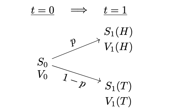Figure 2. One-step binomial model for option pricing.

Here we denote by $p$ ( $1-p$ ) the probability that the stock price end up in “head” (“tail”) branch. We think about these probabilities as reflecting the views of the dealer on how the stock will behave in the future, say according to a complicated statistical analysis. In this sense, they are real world probabilities that are known in the market, that we also inform (as a dealer) our clients with. Now assume that our client contacts us with the intention to buy a call option with a strike that satisfies $S_1(T) < K < S_1(H)$. As an inexperienced dealer we might be tempted to charge our client by reflecting our views on stock price movements by computing the expectation of the option value at the expiry ($t = 1$) based on real world probabilities:

\[\begin{equation} \label{nrnp} \mathbb{E}[V_1] = p V_1(H) + (1-p) V_1(T). \end{equation}\]

By doing so, we might be tempted to think that we found the fair price of this “game”, as on average we expect that our client to make $\mathbb{E}[V_1]$ at time $t = 1$. However, by charging our client the amount in \eqref{nrnp}, we are still exposed to risk. We can see this by focusing on a call option. In this case, there is a non-zero probability that the option will expire in the money such that it’s worth exceeds the amount we charge our client:

\[\textrm{Option expires in the money, so its worth}\quad \Rightarrow \quad V_1(H) > \mathbb{E}[V_1] = p V_1(H),\]

which simply holds because the option is worthless in the “tail” branch $V_1(T) = 0$ and the real-world probability satisfies $p < 1$. To rephare with words, in this world state (the state in which the option is exercised with non-zero value) we owe the client an amount of $V_1(H) = S_1(H) - K$ which is greater than the amount we charge at the inception of the contract, i.e $\mathbb{E}[V_1] = p V_1(H)$.

As market makers (e.g. a dealer), we do not like to take such risks, as we are in the business of selling or buying options without speculating about the future direction of the underlying stock. In this sense, it would not be to our advantage to look at the world states using the real world probabilities of the stock going up $p$ or down $1-p$. Now the ultimate question is how can we minimize our exposure to such risks? A standard approach for this purpose is hedging which amounts to protecting ourselves with a type of insurance/guarantee that will mitigate our potential losses. More concretely, it would be wiser from our perspective to form a portfolio of $\Delta_0$ shares of the underlying at the time we sell our option:

\[\begin{equation}\label{hp} V^{(p)} = \Delta_0 S - V^{(c/p)}. \end{equation}\]

With such a portfolio, we hedge our short position in the option by buying $\Delta_0$ shares of the underlying in order to offset risks against the option. The main goal of the hedging process is to find the optimal parameters $\Delta_0$, i.e. the amount of shares of the underlying we should buy, to determine the value of the option at time $t = 0$.

In the context of the single step binomial model that we schematically represent in Figure 2, the risk originates from the uncertainty associated with the portfolio value that takes up potentially different values in the “head” and “tail” branch:

\[\begin{align} \nonumber V_1^{(p)}(H) &= \Delta_0 S_1(H) - V_1(H),\\ V_1^{(p)}(T) &= \Delta_0 S_1(T) - V_1(T) \label{Vpp} \end{align}\]

where we used a simplified notation for the option value on the right-hand side to generalize the following discussion to both calls and puts. From our perspective, in order to be completely hedged, the portfolio value in \eqref{Vpp} should do not fluctuate between the two states $T/H$. In this case, we know deterministically the value of our portfolio regardless of the future movements of the underlying stock. In other words, we are said to be risk-neutral. The amount of shares we need to buy/sell (at time $t=0$) to realize such a risk-free portfolio can thus be simply obtained by

\[\begin{equation}\label{dhf} V_1^{(p)}(H) = V_1^{(p)}(T),\quad \Rightarrow \quad \Delta_0 = \frac{V_1(H) - V_1(T)}{S_1(H) - S_1(T)}, \end{equation}\]

and is sometimes referred as the Delta-hedging formula. Note that the sign of $\Delta_0$ can change depending on whether we are dealing a call or put option, corresponding to a change in our position to hedge the risk of the corresponding option. Having obtained the optimal amount of shares we need to buy/sell in order hedge our risk, we can turn our attention to our main goal of obtaining the fair value of the option at time $t = 0$. Recall that by equating the potential up and down movements of our portfolio at $t = 1$ we rendered it risk-free. The dynamics of such a risk-free portfolio from $t = 0$ to the final step $t = 1$ should therefore be governed by the “laws” of risk-free rate. In other words, the portfolio value at time $t = 1$ should be just its value at $t = 0$ compounded by the risk-free rate in one unit forward in time:

\[\begin{equation} \label{vp1f} V_1^{(p)} = (1 + r) V_0^{(p)} = (1 + r) \left(\Delta_0 S_0 - V_0\right). \end{equation}\]

Finally, we can use \eqref{vp1f}, \eqref{dhf} and \eqref{Vpp} to solve the fair price we need to charge for the option. After a bit of algebra, we obtain

\[\begin{equation}\label{VO} V_0 = \frac{1}{1+r} \left[ \tilde{p} V_1(H) + \tilde{q} V_1(T)\right], \end{equation}\]

where we defined

\[\begin{equation}\label{rnps} \tilde{p} = 1 - \frac{S_1(H) - (1+r)S_0}{S_1(H) - S_1(T)}, \quad\quad \tilde{q} = \frac{S_1(H) - (1+r)S_0}{S_1(H) - S_1(T)}. \end{equation}\]

Notice that $\tilde{p} + \tilde{q} = 1$ and they are both positive definite thanks to the arbitrage condition \eqref{nac} (see Appendix A). Therefore, $\tilde{p}$ and $\tilde{q}$ can be considered as probabilities. However, they are not the real-world probabilities ($p$ and $q = 1-p$) of the stock going up or down (See Figure 2.). By construction, they are probabilities under which an investor (in our example a dealer) is risk neutral. To further elaborate on these ideas, note that we can re-write the eq. \eqref{VO} as

\[\begin{equation}\label{VOa} V_0 (1 + r) = \tilde{p} V_1(H) + \tilde{q} V_1(T). \end{equation}\]

With $\tilde{p}$ and $\tilde{q}$ treated as probabilities, the right-hand side of \eqref{VOa} does very much resemble an expectation value, similar to the \eqref{nrnp}. The expression \eqref{VOa} then implicates that the value of an option equal to our initial wealth (recall that as a dealer we have an inflow of cash $V_0$ at $t = 0$, when we sell the option), earning a risk-free interest in the money market (e.g. a bank). If this was true and $\tilde{p},\tilde{q}$ were real world probabilities, no one would care invest in the markets as one would make the same amount of money by investing the same amount risk-free. Therefore, the real world probabilities should offer more to be able to convince an investor to risk their money in the stock market:

\[V_0 (1 + r) < p V_1(H) + q V_1(T).\]

In other words, an investor is rewarded in expectation for risking their money in the stock market. $\tilde{p},\tilde{q}$ are therefore called the risk-neutral probabilities. They are probabilities that depend on the price movements of the underlying stock (see Appendix A) with a utility in understanding fair value of the options. It is important to emphasize again that the actual probabilities do not appear in the evaluation of the option in eq. \eqref{VO}. Due to appearance of risk-neutral probabilities, the right-hand side of eq. \eqref{VOa} is sometimes referred as the expectation value of the option under the risk-neutral probability measure. Since, we are agnostic about the real-world probabilities of the stock price going up or down, the pricing methodology we discussed is called the risk-neutral pricing of options.

Appendix A: Risk-neutral probabilities

---

In order to get explicit expressions for the risk-neutral probabilities in terms of the parameters $u$ and $d$ that characterize the stock dynamics within the binomial model, we focus on \eqref{rnps}. Plugging the stock values in the both branch at time $t = 1$, we get

\[\tilde{p} = 1 - \frac{u - r}{u - d} = \frac{r-d}{u-d}, \quad\quad \tilde{q} = 1 - \tilde{p} = \frac{u-r}{u-d}.\]

Notice that by virtue of the no-arbitrage conditions \eqref{nac}, we have $\tilde{p}, \tilde{q} > 0$, making them a valid candidate for probability along with the condition $\tilde{p} + \tilde{q} = 1$.